Recall the tree orchard site we’ve been looking at. This site is relatively flat with distinct (potted) objects.
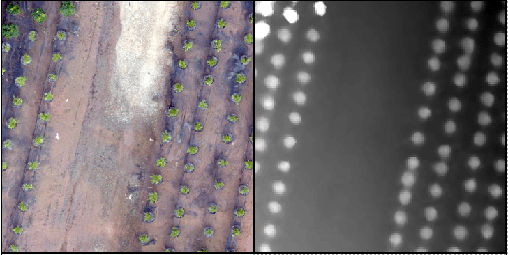
In this lab, I will attempt to lead you through an R-based analysis with the goal of segmenting the landscape (individual potted plants).
INPUT DATA:
Lab data is linked HERE. Use the download link at the top of the page and save the file as “Nov30_2017.zip”. Copy the compressed file to your c:\drive working directory and then right-click>extract all to uncompress. You should have two folders; one called “InputPhotos” and another called “PhotoscanOutput”. You will be using the files found in the PhotoscanOutput folder.
- clpSG_Ortho.img: Photoscan orthophoto
- clpSG_TerrainModel.img: Photoscan terrain model
- clpSG_PointCloud.las: Photoscan point cloud
PROCESSING IN R (entire script pasted at the end of this page):
You will be using the R code I demonstrated in class last Friday. The processing workflow relies on the lidR library (documentation here). Lets look at it bit-by-bit…
In this first part, you install and/or load required libraries. You will use the EBImage, lidR, and raster libraries. Start the most recent X86 version of R (Start > All Apps > …). If a library is not already installed on the machine, you can do so by Packages > Install Packages.
#####Install/Load libraries
source("https://bioconductor.org/biocLite.R")
biocLite("EBImage")
library(EBImage)
library(lidR)
library(raster)
Yes, we need set your working directory.
#####Specify Working Directory
#####This should point to the directory in which your *.las resides
setwd("C:/temp/Nov30_2017/PhotoscanOutput/")
Read the LAS file into the “my_data1” R object. Note that there is a writeLAS command too.
#####Read LAS file
#####https://rdrr.io/cran/lidR/man/readLAS.html
my_data1<- readLAS("clpSG_PointCloud_th001.las")
##make note of min/max X Y Z:
##make note of Num. of point records
summary(my_data1)
The first step in the process is to classify the site’s ground points.
#####Classify ground points
#####https://rdrr.io/cran/lidR/man/lasground.html
#####ws: sequence of window sizes to be used in filtering ground points
ws = seq(0.75,3, 0.75)
#####th: sequence of threshold heights above the surface to be considered a ground return
#####this step may take some time to run...
th = seq(0.1, 1.1, length.out = length(ws))
lasground(my_data1, "pmf", ws, th)
plot(my_data1, color = "Classification")
#####make a back up of the my_data1 object
my_data1_bak<- my_data1
Here, you compute the terrain model (the bare ground model). I have you run the process twice. Once with a 0.9 meter resolution and another with a 0.5 meter resolution. Do you see any issues with the results?
#####compute digital terrain model (DTM), this is the surface minus features sitting on top
#####https://rdrr.io/cran/lidR/man/grid_terrain.html
dtm1 = grid_terrain(my_data1, res=0.9, method="knnidw", k=10, keep_lowest=TRUE)
plot(dtm1)
#####process w/ smaller ground resolution
my_data1<- my_data1_bak
dtm2 = grid_terrain(my_data1, res=0.5, method="knnidw", k=10, keep_lowest=TRUE)
plot(dtm2)
Up to this point, the my_data1 surface is an irregular surface that contains the bare ground, pots, plants, and any other object sitting on top of the ground. The dtm2 surface contains only the bare ground points. The lasnormalize command differences the first and second images, and the result is a normalized surface.
#####normalize point cloud: subtract DTM from point cloud; value 0 represents ground-level
#####https://rdrr.io/cran/lidR/man/lasnormalize.html
lasnormalize(my_data1, dtm2)
#####my_data1 now contains the normalized heights
##make note of min/max X Y Z:
summary(my_data1)
plot(my_data1)
my_data1_bak2<- my_data1
The gridcanopy command returns the high points in the my_data1 surface. The chm results is too coarse. The process is rerun with a resolution of 0.05 meters and stored as chm2.
#####create grid canopy
#####for each grid, returns the highest point
#####https://rdrr.io/cran/lidR/man/grid_canopy.html
chm = grid_canopy(my_data1, res=0.25, subcircle = 0.2)
plot(chm)
my_data1<- my_data1_bak2
chm2 = grid_canopy(my_data1, 0.05, subcircle = 0.025)
plot(chm2)
#####notice the redefined canopies
chm2 = as.raster(chm2)
The next processes smooths the canopy height model (removes some of the internal holes
#####smoothing post-process (2x mean)
kernel<- matrix(1,3,3)
chm2a = raster::focal(chm2, w=kernel, fun=mean)
chm2a = raster::focal(chm2, w=kernel, fun=mean)
raster::plot(chm2a, col=height.colors(50))
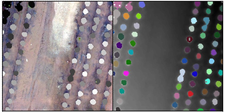
These last commands perform the segmentation process.
#####segmentation process
#####https://rdrr.io/cran/lidR/man/lastrees.html
crowns = lastrees(my_data1, "watershed", chm2a, th=0.25, extra=TRUE)
contour = rasterToPolygons(crowns, dissolve=TRUE)
tree = lasfilter(my_data1, !is.na(treeID))
plot(chm2, col=height.colors(50))
plot(contour, add=T)
Use the last command to write the R objects out as a TIF you can load into ArcMap!!!
raster::writeRaster(crowns, filename="crowns1.tif", format="HFA", overwrite=TRUE)
The raster you export is a multi-layer raster. Use the Raster Calculator to quickly convert the raster to an integer raster – one that does have an attribute table. Load the raster you exported above and the orthophoto into ArcMap. It should look something like this…
There is no deliverable for this lab.