Click HERE to access the lab data repository!!! You can click HERE too Nothing will happen If you click here.
Download OcNF_Data.gdb2.zip from the data repository and set up your project workspace on the E:\ drive (even though the lab document or screen shots may reference the c:\ drive). Start ArcMap but don’t load any data…
<Begin Discussion…>
- Something is wrong with your project workspace, maybe
- A-Z, a-z, 0-9, and “_”
- NO strange characters allowed in any part of your project workspace path and NO strange characters allowed in any part of your GIS layer names
- What bits of information do the OCNF GIS layers contain?
- Notice no attribute table for the raster topo map
- We have tabular data that is not associated with any spatial entity, yet…
- Layer Symbolization
- Join external table to GIS layer
- Dissolve features
- Map layout creation
<End Discussion…>
SAVE YOUR PROJECT OFTEN (FILE > SAVE or CTRL-S)!!!!
THE COMPSTAND LAYER
CompStands: This is our forest-level data layer. Each polygon is attributed with Tract, Compartment, Stands, UniqID, record, StandKey, and GISAcres. (right-click on the layer > Open Attribute Table)
- StandKey is your ‘common ID’ field – this the field that uniquely identifies each polygon. You will use this information to join any field data
- Compartmnt identifies the management unit within the forest; there are 7 unique compartments within the forest
- Stands is a sequential number within each Compartmnt
- UniqID is another field that uniquely identifies each polygon feature; it is a combination of the Compartmnt field and the Stands field
- Record contains a sequential number for the entire forest; 1, …, 896
- GISAcres is a field to store each polygon feature’s GIS-calculated acreage.
- You can populate this field by: Open the Attribute Table > Right-click on this field > Calculate Geometry >> …
- Shape_Length and Shape_Area are added by the software. You can not modify these fields.
SYMBOLIZATION
Right-click on the layer CompStands > Properties > click the Symbology tab (see screenshot below)
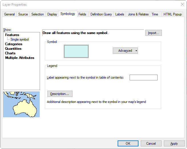
To symbolize the polygon features based on the categorical variable (see screenshot below)
- Click Categories in the left pane > select the Value Field Compartmnt > Hit the ‘Add All Values’ button at the bottom > Hit OK

For now, make sure the drawing order in the TOC is as follows:
- point layer
- line layers
- polygon layers (soils turned off – un-checked)
Hit Quantities in the left pane (screenshot above) to symbolize the polygon features based on a continuous variable
Symbolize this layer by each of these attributes to get a feel for what these attributes represent.
JOIN EXTERNAL TABLE TO COMPSTANDS LAYER
These stand boundaries will not change often – these are the units at which management activities are performed. There is, however, information about each stand that does change periodically. It makes more sense to provide this information as a TABLE and to JOIN this table to the CompStand layer. When the inventory information changes, I unjoin the current table and then repeat the join using the updated table.
To see the TABLE layers in your project, you must List the Layers by Source in the Table of Contents (the second icon from the left).

Right-click on Stand_Info layer > select Open to view the TABLE. The fields of interest are StandKey, ForestType, StandAge, StandBAAC, StandCUFTA, ExtabYr.
- StandKey is your CommonID field for this table. It links one-to-one with the polygon features in the CompStands layer.
- ForestType is a categorical descriptor of forest type
- StandAge is a numeric field containing age. You need to update this field each uear. (Current Year – EstabYr)
- StandBAAC is a numeric field containing basal area per acre measured in square feet
- StandCUFTA is a numeric field containing the cubic foot volume per acre
- EstabYr is a numeric field containing the year each stand was established.
To join the information in our Stand_Info table to the polygon features in our CompStands layer, you do the following:
- Unselect all records in CompStands and Stand_Info
- Open the attribute table
- Table Options > Clear Selection
- Open the Stand_info table
- Table Options > Clear Selection
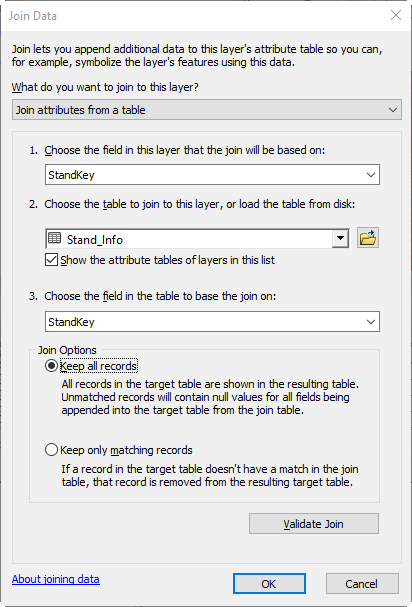
- Right-click on the CompStands layer in the Table of Contents > Joins & Relates > Join
- StandKey (this is the common ID field in the CompStands layer)
- Stand_info (check the box “Show the attribute tables…”; this is the external table you will join to your spatial data)
- StandKey (this is the common ID field in your external table)
- Tick the box next to “Keep all records”
- OK
View the CompStands attribute table and scroll to the right to see the joined fields. This join is only present in this project. If you load CompStands into another project, you will not see these joined fields in the attribute table. Joined tables are only present in the project in which you perform the join – they do not carry over to other projects.
DISSOLVE COMPSTANDS TO CREATE A NEW LAYER TO REPRESENT THE 7 DIFFERENT COMPARTMENTS
The DISSOLVE command in GIS aggregates features based on a specified attribute. Before you run this command, unselect everything in the CompStand layer. Use the search functionality within ArcGIS to find this tool. Select Search from the ArcGIS Windows menu and then type ‘dissolve’ in the search box. Click on the entry called “Dissolve (Data Management)”.
The DISSOLVE tool allows for the calculation of statistics from fields in the input layer. After the join, our input layer, CompStands, has fields EstabYr, StandBAAC, and StandCUFTA. When you specify a field and a statistic type (in the Statistics section of the DISSOLVE dialog), the results will be stored in the attribute table of the output layer.
In this example (screenshot below):
- I dissolve on the Compartmnt field in the CompStands layer
- The new layer will be called CompStands_Compartmnt and is saved in my working directory
- The software adds a field in the output layer that contains the mean, min, and max EstabYr, StandBAAC, and StandCUFTA. To do this, you must select the field three times and assign the mean statistic to one, the min statistic to another, and the max statistic to the remaining.
- I unchecked the “Create multipart features” button.

Look at the output layer’s attribute table to make sure those min, max, and mean statistic fields are present.
ADD GISACRES FIELD TO YOUR DISSOLVED COMPARTMENT LAYER and CALCULATE ACREAGE
Open the dissolved layer’s attribute table and
- Table Options > Add a new field
- Call it “GISAcres” and make it a FLOAT type
- Right-click on your new GISAcres field > Calculate Geometry
EXPORT YOUR ATTRIBUTE DATA FOR SUMMARIZING AND GRAPHING
Open your CompStands attribute table > Table Options > Export > hit folder icon
- Save as type: Text File
- Name: CompStands_information.csv
- Look in: change to your working directory (make sure you are not pointing to the .gdb)
- No need to add to project after you hit OK
You now have a new CSV file in your working directory you can open in Excel, R, or any other data analysis package.
CREATING A MAP LAYOUT
Up to this point in the lab, you have been working in the Data View (View > Data View). This is the view mode you you’ll use when processing data. When you are ready to create a map, you will switch to Layout View (View > Layout View).
Enter into layout mode (View > Layout View)
- Add north arrow (Insert pull-down-menu > North Arrow)
- Add scale bar (Insert pull-down-menu> Scale Bar)
- Add text (Insert > Text)
- Add legend (Insert > Legend)
- Add title (Insert > Title)
Save your project.
Lab deliverables
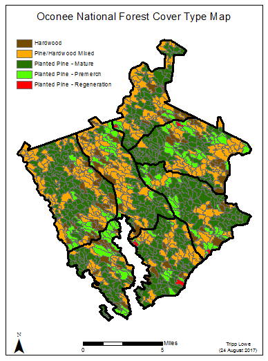
Task 1 (10 points): Create a map layout showing:
- (1 pt) The dissolved compartment layer symbolized with a clear fill and a thick black outline shown on top
- (2 pts) The CompStands layer symbolized by ForestType
- Hardwood -> brown
- Pine/Hardwood Mixed -> orange
- Planted Pine – Mature -> dark green
- Planted Pine – Premerch -> light green
- Planted Pine – Regeneration -> red
- UNTICK THE BOX NEXT TO “<all other values>”
- (7 pts) North arrow, scale bar, legend showing only the information for CompStands, Title, and a text box with your name and the current date.
- Each map element you add has a ‘right-click > Properties’ where you can adjust map units, font, color, etc.
- File > Export Map > save as JPEG into your working directory.
- Upload your map layout export to the Lab 2 ELC folder.
Task 2 (5 points): Create a short screen cast documenting the process of joining an external table to an existing GIS layer.
- Save your lab ArcMap project and then open a blank instance of ArcMap (File>New)
- Start your recording now.
- You will need to
- load the CompStands layer and the external Stand_Info tabular data you used in lab
- join the table
- symbolize the CompStands layer on the StandBAAC field using Quantities>Graduated colors>Quartile (3 classes)
- Stop recording.
- Name this MP4 “JoinExternalTable.mp4”
- Upload this to the Lab 1 assignment dropbox