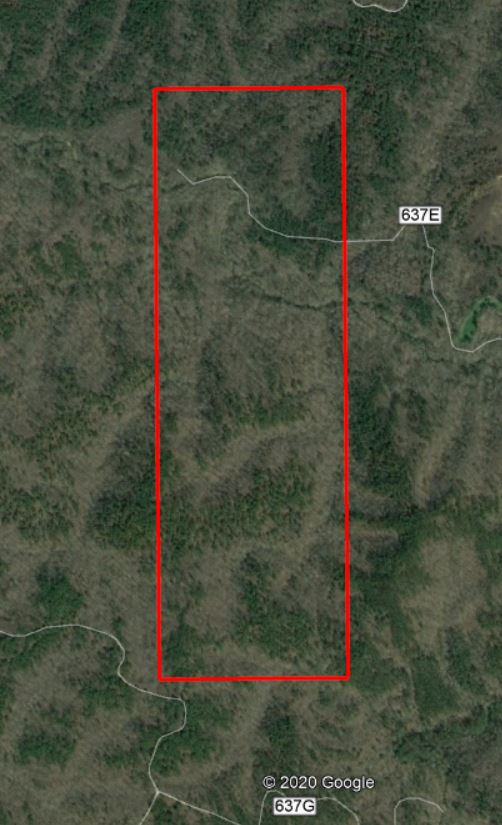
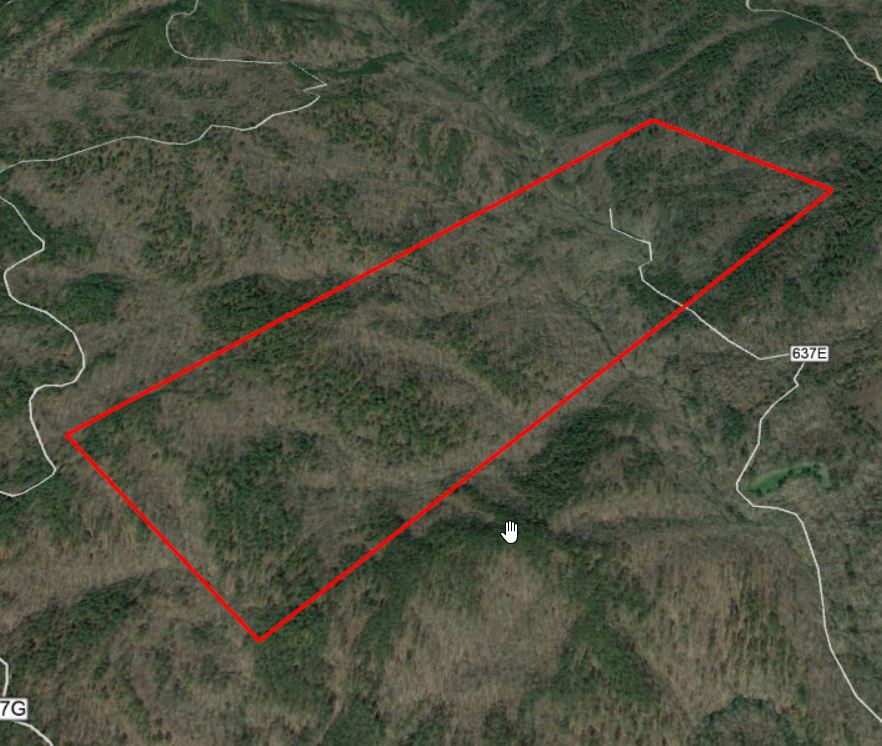
Lets continue with the Talladega National Forest LiDAR dataset… I have provided a link to a KML of the LiDAR panel 625065 extent. Give the site a look in Google Earth to get a better feel for the site (Figure 1). A stream in the northern part of this site flows in an east-west direction. Terrain in both the southern and northern portions slope inward towards this stream (Figure 2). Land cover consists of mature hardwood and mature natural pine.
Let me step through the code from Monday piece by piece. I am following the general work flow for “Rasterizing perfect canopy height models” ( https://github.com/Jean-Romain/lidR/wiki/Rasterizing-perfect-canopy-height-models ). I will provide links to the docs as comments in the code if you need help with syntax.
###Load required libraries
library("lidR")
library("rgdal")

###You need to change this path to match where you save the data
mypath<- "V:\\Krista_LiDAR\\Tripp_LiDAR"

###Store LAS filename as a variable
ttyfn<- "625065.las"

###Read LAS file and store as the R object 'tty'
tty<- readLAS(file.path(mypath,ttyfn))

###Report header information
summary(tty)
###General statistics of LiDAR attributes, two examples...
unique(tty$Z)
max(tty$Z)

###The available LiDAR attributes are (see names section of the summary)
###See ASPRS documentation, table 4.7
###https://www.asprs.org/wp-content/uploads/2010/12/LAS_1-4_R6.pdf
### X Y Z gpstime Intensity ReturnNumber NumberOfReturns ScanDirectionFlag EdgeOfFlightline Classification Synthetic_flag Keypoint_flag Withheld_flag ScanAngleRank UserData PointSourceID
Nothing new up to this point – you have loaded the point cloud into R and stored it as the R object tty.
Next, to speed processing, lets clip out a small part of the point cloud. I created this shapefile in ArcMap. I loaded the LAS into a blank ArcMap document; this matches the data frame coordinate system with the LAS file (Alabama State Plane East, NAD 1983). Next, I created a new polygon shapefile, making sure to set the spatial reference to Alabama SPE, and drew the polygon myself.
A practical application… Imagine that we have sample plots located in this area and we want to relate the ground measurements to the LiDAR data. We can use this same approach to extract the LiDAR metrics (average height, max/min height, Xth percentile height, slope, aspect, etc) for our samples.
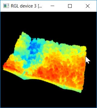
###shapefile is stored in the same folder as the other data
shppath<- mypath
###This is the name of the clip shapefile
shpname<- "ClipSection_TNF"
###Load the shapefile
shape_spdf<- readOGR(dsn = shppath, layer = shpname)
###reference the first polygon
shppoly<- shape_spdf@polygons[[1]]@Polygons[[1]]

lascliptty<- lasclip(tty, shppoly)
plot(lascliptty)
Somebody else flew this LiDAR mission and I do not have documentation about how this layer has been processed. Part of this workflow relies on each point’s Classification (recall this is one of the LAS attributes). To ensure we are working with proper classifications, we’ll reset everything to 0.
lascliptty$Classification<- as.integer(0)
Before we can normalize the point cloud, we must first identify the ‘ground’ points. In this code, we’re using the PMF algorithm ( https://rdrr.io/cran/lidR/man/lasground.html ).
###https://rdrr.io/cran/lidR/man/pmf.html
ws<- seq(3,12,3)
th<- seq(0.1, 1.5, length.out = length(ws))
###lasground is the lidR function to classify the ground points
lasdpmf<- lasground(lascliptty,pmf(ws,th))
plot(lasdpmf, color="Classification")

unique(lasdpmf$Classification)

###Count the number of fround-classified points
sum(lasdpmf$Classification == 2)
Notice the output of the last line. The unique Classification values are “unassigned” (1) and “ground” (2). Also, there are 138,473 ground points.
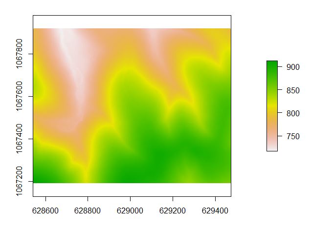
In the next segment of code, you create the digital terrain model. Recall that you classified the ground points in the section above. The grid_terrain command uses the ground-classified points to interpolate the raster surface.
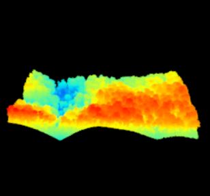
The DTM is then used to normalize the original point cloud. Think of this step as subtracting the DTM values from the original Z values – moving from a measure of elevation to a measure of height above the immediate ground surface.
###create the digital terrain model
###https://rdrr.io/cran/lidR/man/grid_terrain.html
dtm<- grid_terrain(lasdpmf, 1, knnidw(k=6L, p=2))
plot(dtm)
###save the DTM out as a raster you can load into ArcMap
writeRaster(dtm,filename=file.path(mypath,"dtm.tif"), format="GTiff",overwrite=TRUE)

###normalize the point cloud
###https://rdrr.io/cran/lidR/man/lasnormalize.html
lasdpmf_norm<- lasnormalize(lasdpmf,dtm)
plot(lasdpmf_norm)
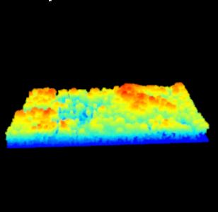
We expect that all values in the normalized point cloud are >= 0. A quick view of the point cloud headers, use the summary(lasdpmf_norm) reveals that the minimum Z value is -2.8. In the code below, we use the lasfilter function to create a new R object, lasdpmf_norm_gt0, that stores all non-negative points.
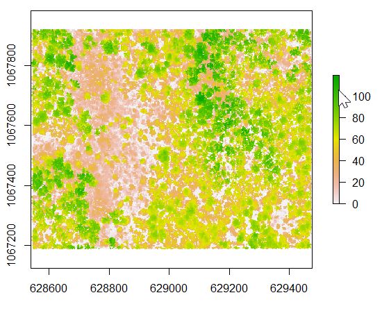
###remove all of the negative heights by creating a new R object that contains all points whose Z is >= 0
###https://rdrr.io/cran/lidR/man/lasfilter.html
lasdpmf_norm_gt0<- lasfilter(lasdpmf_norm, Z >= 0)
summary(lasdpmf_norm_gt0)

###Canopy height model (CHM)
###https://rdrr.io/cran/lidR/man/grid_canopy.html
chm_pmf0205<- grid_canopy(lasdpmf_norm_gt0, 02.5, p2r(0.5))
plot(chm_pmf0205)

###export the CHM as a raster file to load into ArcMap
writeRaster(chm_pmf0205, filename = file.path(mypath,"chm_pmf0205.tif"),format="GTiff",overwrite=TRUE)
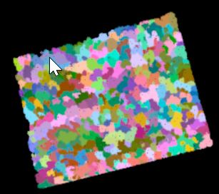
######detect individual tree tops and crowns
###https://rdrr.io/cran/lidR/man/lmf.html
ttops <- tree_detection(lasdpmf_norm_gt0, lmf(20, 35, "circular"))
plot(ttops)

###https://rdrr.io/cran/lidR/man/lastrees.html
##############
############## This next line was the reason the plots did not work out
############## I reference the wrong R object.  Instead of lasd_n<- ... it
############## should be lasdpmf_norm_gt0<-...
###NOT THIS >>>>> lasd_n<- lastrees(lasdpmf_norm_gt0,mcwatershed(chm_pmf,ttops))
###but this>>>
col<- pastel.colors(250)
lasdpmf_norm_gt0<- lastrees(lasdpmf_norm_gt0,mcwatershed(chm_pmf0205,ttops))

####if mcwatershed above throws an error, then try this below
lasdpmf_norm_gt0<- lastrees(lasdpmf_norm_gt0, li2012(R=3, speed_up = 5))

###############
###############
###https://rdrr.io/cran/lidR/man/silva2016.html
crowns = silva2016(chm_pmf0205,ttops)()
###plot the point cloud and colorize by segmented crowns
x = plot(lasdpmf_norm_gt0, color = "treeID", colorPalette = col)
add_treetops3d(x, ttops)

###Export the crown segments as a raster
writeRaster(crowns,filename=file.path(mypath,"treecrown.tif"), format="GTiff", overwrite=TRUE)
###Export the tree tops
writeOGR(obj=ttops,dsn=mypath,layer="treetops",driver="ESRI Shapefile", overwrite = TRUE)
One last thing… Lets calculate statistics for each of our tree segments. Calculate the mean, maximum, and minimum values for each segment based on the CHM value (r) and the un-normalized values (zr). This is similar to using ArcMap’s Zonal Statistics As Table command.
#####Statistics for groups of trees
###z references the CHM value
###zr references the original elevation value
myMetrics = function(z, zr)
{
  metrics = list(
    zmean = mean(z),
    zmax  = max(z),
    zmin  = min(z),
    zrmean = mean(zr),
    zrmax  = max(zr),
    zrmin  = min(zr)
  )

  return(metrics)
}
treestats<- tree_metrics(lasdpmf_norm_gt0, myMetrics(Z, Zref))
metricsOut<- "TreeMetrics.csv"
write.csv(treestats, file= file.path(mypath,metricsOut))