Your task for this lab is to create marketing material for a timberland parcel being advertised on the Land Watch website. You will 1) locate teh parcel in QPublic, 2) download multiple years worth of aerial photos, soils, hydrology, watershed boundaries, and roads from the NRCS Geospatial Data Gateway, 3) import the data into a file geodatabase, and 4) output a series of maps for the site. (No digitizing in this lab!)
Due-diligence Mapping
Due-diligence mapping is the term I use when I create a series of maps showing all available data for a site. Once you have all of the data stored locally and loaded in ArcMap and all of the map layout elements inserted, you turn a base layer on and export, turn that layer off and a new one on and export, then turn that layer off and another on and export, and so…
Prepare your workspace…
As always, create a new folder to store all of this week’s GIS data. Make sure you know the path of this workspace. It should be something like E:\DueDiliLab\. You will need to know where it is. You can go ahead and create a file geodatabase, but there is no need to create any feature classes since the data you will use already exists – you will be importing the data, not creating new data for this lab.
Go ahead and open ArcMap and save the project to this workspace (File >> Save As). Normally, you would also set the data frame coordinate system (View >> Data Frame Properties >> Coordinate System tab), but you haven’t figured out which UTM zone you will need to use. It is best to hold off on this for now.
The lab…
Our client, Matre Forestry Consulting, has contracted us to put together a mapping package for a property they have for sale somewhere in Georgia. The property is listed on the web at Cotton Boat Shoals.
You will do the following:
- Download the KML from QPublic and import (KML to Layer) it as a feature class in ArcMap
Use the Feature to Polygon tool to convert the layer you just imported to a polygon shapefile- Download your data from the NRCS Geospatial Data Gateway, unzip, and load into your Arcmap project
- Clip the images to your surrounding site
- Zoom into your property and then zoom out some so you can see the surrounding area
- (right-click on raster layer >> Data >> Export Data), saving the output to your file geodatabase
- Symbolize and label the NRCS roads and hydrology; prepare your layout
- Turn on your boundary and the first image, export JPEG (File >> Export), turn off the first image
- Turn on the second image, export JPEG, turn off the second image
- Repeat for each NRCS raster
You must find the property before you can begin
The goal here is to figure out where this property is located. Most helpful would be XY coordinates, street address, road intersection, or a visual cue and a general location to help you find the property in Google Earth.
- Any information on the LandWatch website to help?
- Any information on the consultant’s website?
Set the data frame coordinate system
At this point, you should know what county you are in. Have you figured out what UTM zone you need to use? If you are east of Atlanta, use UTM zone 17N and use UTM zone 16N if you are west of Atlanta.
In ArcMap, open the Coordinate System tab in the Data Frame properties (View >> Data Frame Properties) and set the proper coordinate system for this site. Save your project.
Download the parcel KML from QPublic
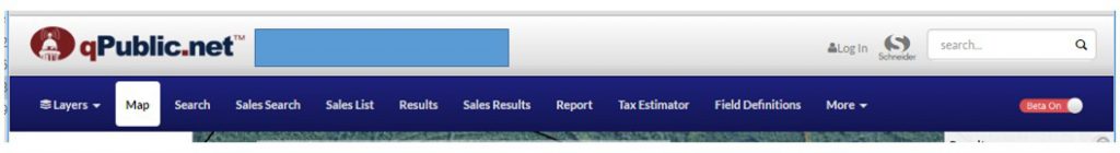
Now that you know the county and have at least a general idea of where the property is located, visit the appropriate county QPublic site (hint: google <county> QPublic) and download the parcel’s KML. QPublic is in the process of updating their web interface and it appears it does not provide an easy KML download link so you need to turn the “Beta Off” (upper right corner).
Import KML, convert to polygon, and import into FGDB
Run the KML to Layer routine to import the QPublic data into ArcMap. Use the Search box to find this tool (Windows >> Search). This tool creates a line-type feature class, yet you need a polygon. Change the layer’s color, the default is white. Run the Feature to Polygon tool to do the conversion for you. Make sure you specify the FGDB you created at the very start as your output location and you can name it MyBoundary. You now have two layers in your ArcMap project. Center on one of the layers (Right-Click >> Zoom to Layer) and then type “1:15840″ in the scale box to set the scale to 1″ to 660′ (1” to 10ch). Save your ArcMap project (File >> Save)
Download your layers from the NRCS Geospatial Data Gateway
Give the NRCS Geospatial Data Gateway document a read for how to navigate this site. You need to download the following:
- Hydrography (rivers and streams)
- 12 Digit Watershed Boundary (HUC 12 watershed boundary)
- Digital Raster Graphic County Mosaic (georeferenced USGS Topo map)
- Soils from the Web Soil Survey
- 2007 NAIP (georeferenced color aerial from 2007)
- 2009 NAIP (georeferenced color aerial from 2009)
- 2010 NAIP (georeferenced color aerial from 2010)
- 2013 NAIP (georeferenced color aerial from 2013)
- 2015 NAIP (georeferenced color aerial from 2015)
- 2017 NAIP (georeferenced color aerial from 2017)
- 2019 NAIP (georeferenced color aerial from 2019)
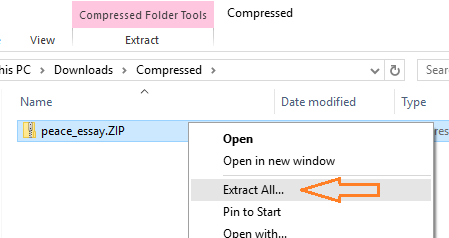
Each of these downloads are compressed (zipped) files. You must unzip each. There is an additional compressed file inside the soil folder – uncompress this one as well. Recall that you unzip a file from Windows Explorer (right-click >> Extract All…) then in the dialog that appears, type in the path of the working directory you created at the beginning – don’t let Windows decide where your data is stored!
After extracting all of the data, your working directory will look like this: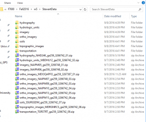
Load your NRCS layers
The uncompressed layers are scattered between 7 folders.
- Load the NRCS orthophoto raster layers
- Load vector layers nhd24kst_l_ga….shp and nhd24kwb_a_….shp layers from the hydrography folder
- Load vector layer wbdhu12_a_ga….shp from the hydrologic_units folder
- Load the vector soils layer from the Web Soil Survey
- Load the raster digital raster graphic (DRG)
- Load the transportation vector layer
Clip the rasters and save in the FGDB
Just in case, center on your boundary layer (right-click on your boundary layer >> Zoom to Layer) and then zoom out to 1:15840 (type 1:15840 in the scale box).
- Extract the rasters: right-click on a raster >> Data >> Export Data..
.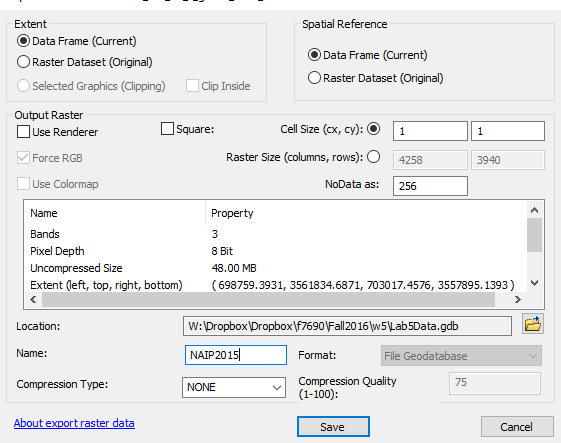
- Tick ‘Data Frame (Current)’ under Extent and Spatial Reference at the top
- Navigate to your FGDB in the Location section
- Name the new file something intuitive
- Hit Save
- Repeat these steps for all downloaded rasters
- Ensure you tick DATA FRAME (CURRENT) each time you export an image and you specify your working FGDB as the output location
- Yes, add the layer when prompted
Use a dirty clip to extract the vectors
The lakes, rivers, soils, roads, and watershed vector layers cover the entire county. Lets use a dirty clip to make the data a bit easier to handle.
Turn on the soils layer and turn off everything else. Grab the SELECT FEATURE tool (to the right of the blue right arrow) and draw a box around all of the soil polygons you see on your screen. The selected polygon features are blue. Now:
- Right-click on the soilmu_a_ga259 layer >> Data >> Export Data
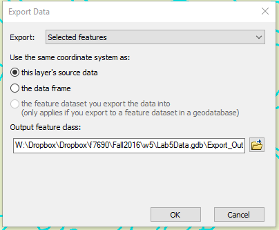
- Use the file/open dialog to navigate to your FGDB,
- Save As Type should be “File and Personal Geodatabase Feature classes”
- name it soils and SAVE/OK/YES
- Use the file/open dialog to navigate to your FGDB,
- Repeat for the wbdju12_a_ga… layer; name it watershed_huc12
- Repeat for the nhd24kwb_a_ga… layer; name it lakes
- Repeat for the nhd24kst_l_ga… layer; name it rivers
- Repeat for the street100k_l_ga… layer; name it roads
Save your project
Organize the layers in your ArcMap project
At this point, you probably have quite a few layers shown in the TOC. It is a good idea to remove the layers you won’t be using. Keep the polygon parcel boundary, the dirty-clipped vectors, and the rasters you exported to your FGDB. Remove all of the other layers. Save your project.
Prepare your map layout
- Enter Layout Mode
- Zoom to your property boundary layer and then set the map scale to 1:12000
- Add the required map element
- Make sure you have a text box in which you enter the image source
- Symbolize your boundary layer
- Symbolize your road, river, and lake layers
- Label the roads (open the road properties >> goto Label tab >> …)
- Tick the Label Features box in the upper left
- Specify the road name field as the label field
- Adjust the label font and color (click the symbol button)
- Use either white or black for the label color
- Make sure the font size is not so large that it distracts from the map
- Label the rivers layer with the river name
Save your project
Export maps
In this last step, you keep the boundary, road, river, and lake layers visible. To get started, turn off all the other layers.
- Turn the NAIP2007 image on, adjust the source text, export the map, turn the layer off.
- Repeat for all other rasters
- Prepare the soils map export
- Symbolize the soils layer as hollow with a light brown or burnt orange outline color.
- Label the polygons based on the MUSYM field, match the label color to the polygon outline color.
- Turn the NAIP2019 layer on
- You should see the image and the soil boundaries and the soil labels as well as the road, river, and lake layers
- Export the map
Save your project. Make sure you know where you saved your project, you WILL use it later on.
Upload the following to the ELC dropbox by midnight, next Thursday.
- Multiple maps (JPEGS) with property boundary, roads, rivers, streams overlaying the 2007, 2010, 2013, 2015, 2017, 2019, USGS Topo, and the soil map overlaying the NAIP 2019 ortho. Name the output <LastName>_<image source>