Lab 3 to upload to ELC by next Thursday at midnight. Browse the properties referenced on the AFM property search page (https://americanforestmanagement.com/real-estate/property-search) for examples of ‘good’ maps – maps that you think convey the idea that this is the property for you! Most of the property pages I’ve looked at have a Related Documents section to the right of the page with links to aerial photo, topo, or location maps. I want you to find one map that contains something that you want to do in your maps. Copy into a Word document the URL, a screen shot of the map, and what it is that you want to be able to do that you see in the map – be specific. Upload this document to ELC. Do this after you work through the rest of the lab. I
Lab 3… You will be working in this project next Wednesday, so make sure you save everything to your working directory and that you copy this working directory up to your network space when you finish today.
You have been contacted by a client group who needs maps of four parcels scattered across three counties.
- Two parcels in Walton county under the ownership “Dallyville LLC” (34.79 acre and 125 acre parcels) (figure 1)
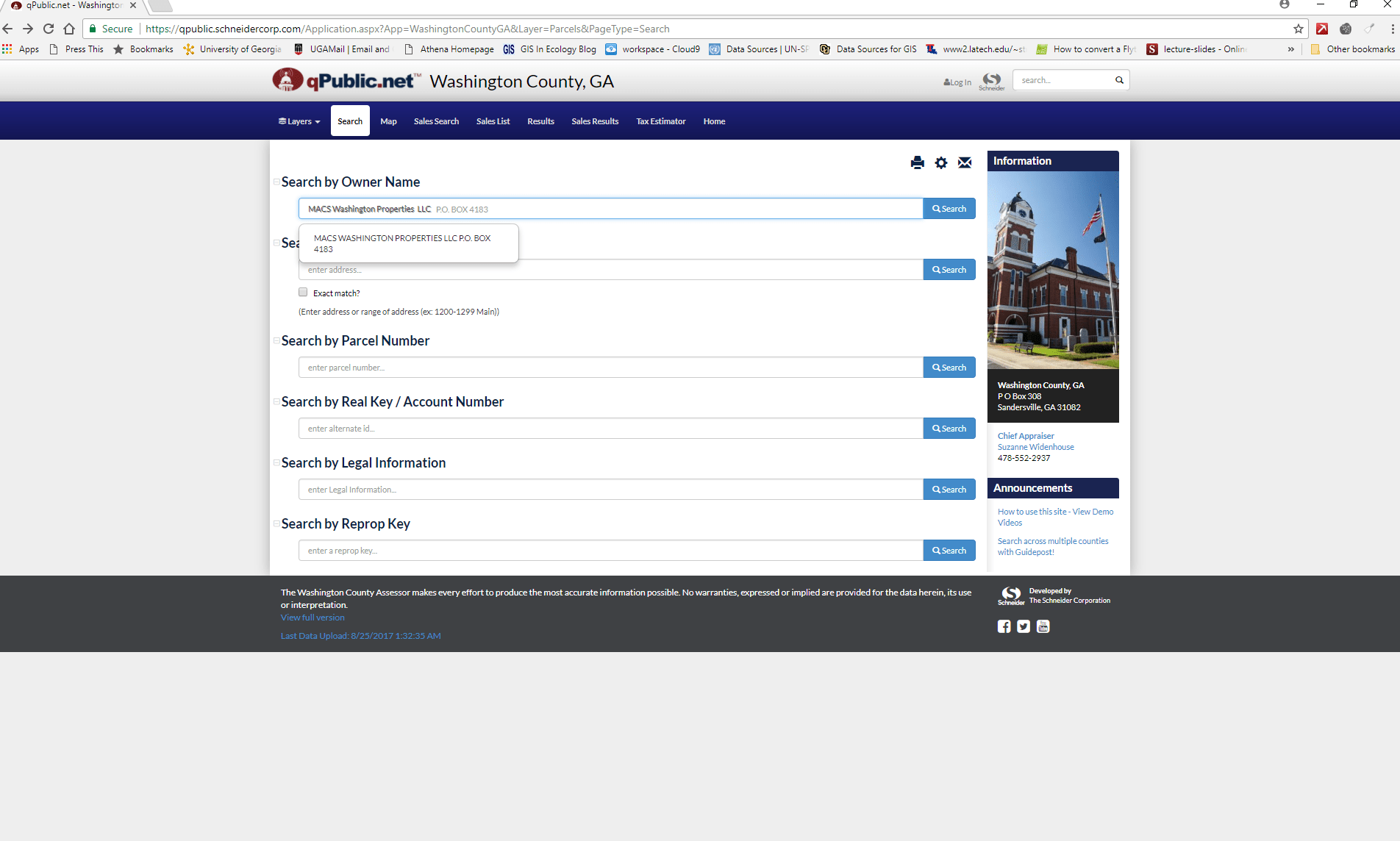
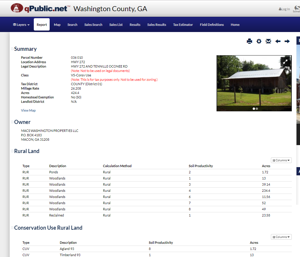
- One 424.4 acre property in Washington county under the ownership of “MACS Washington Properties LLC” (figure 2)
- One 331.74 acre property in Elbert county under the ownership of “Broad River Properties LLC” (figure 3)
Figure 1. Dallyville, LLC. land holdings in Walton county, Georgia.
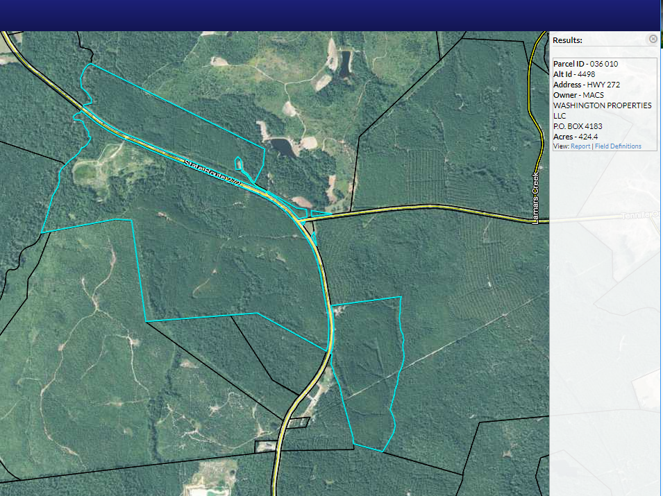
Figure 2. MACS Washington Properties, LLC. land holding in Washington county, Georgia.
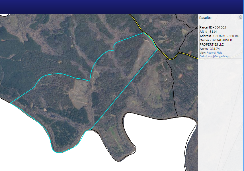
Figure 3. Broad River Properties, LLC. holding in Elbert county, Georgia.
Processing Overview
- Create your working directory
- Download KMLS from qPublic
- Save the qPublic tax record for each property
- Run the ArcMap command KML TO LAYER to convert each KML file (from step 2) to an intermediate feature class
- Create one new file geodatabase called “PropertiesLLC” in which you will save all of the GIS layers you create
- Import the feature classes (from step 4) into the file geodatabase (from step 5)
- Run the ArcMap command MERGE (DATA MANAGEMENT) to combine the polygon features from the different layers (created in step 6) into a single layer called “PropertyBoundaries”
- Use the ArcMap PROJECT command to mathematically transform the Lat/Long boundaries to a projected coordinate system
At the end of this lab, you will have an ArcMap project with one GIS layer. This polygon feature class layer will contain all of your client’s property boundaries. You will continue on this project next week when you will determine the acreage of the different cover types and generate summaries for the properties.
You will see text outlined in orange throughout this lab. This is my way of indicating that you are about to have to do something. I have also included a written narrative with plenty of screenshots.
A final word on this lab… At the start, you download three of KML files and then import them into their own file geodatabase – you have three of these in your working directory. You then import these feature classes into a file geodatabase that you create – one file geodatabase with three feature classes. Next, you merge these three feature classes into one. When working on projects where there are multiple, non-adjacent land holdings, the GIS operator has to decide if it is best to work with individual feature classes or merge them all together (like we do in this lab). My advice is to merge the layers and process the one file instead of having to process three files – fewer chances for error.
————————————————————————————-
Set up working directory
Create folder on the C:\ drive called “lab3properties”
qPublic.net (do these steps for each of the three properties)
Counties in Georgia, Colorado, Connecticut, Kentucky, Louisiana, and South Carolina provide access to online GIS parcel information through qPublic.net. This services enables users to search parcel-level records and, in many cases, download GIS-ready parcel boundaries. Please note, however, some counties provide this service free-of-charge while others require a daily/monthly/yearly per-county subscription (the daily subscription fee is $10 per county). For more information, visit qpublic.net.
NAVIGATING THE QPUBLIC SITE (in PICTURES)
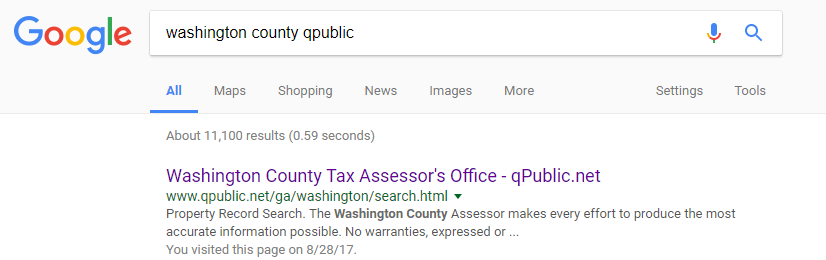
- Google is a good place to start to find your county’s qPublic site
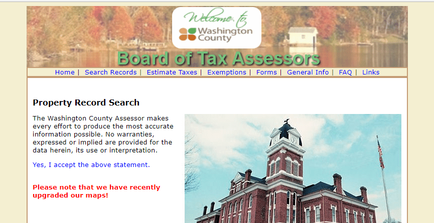
- Accept the statement in blue…
- If the site is NOT behind a pay-wall, enter your search criteria and hit the search button
If the site IS behind a pay-wall, you must register and pay before entering the site. qPublic offers a reasonable 10$/day subscription level. - Use the REPORT tab (along the top of the page) displays tax-related information for the property query
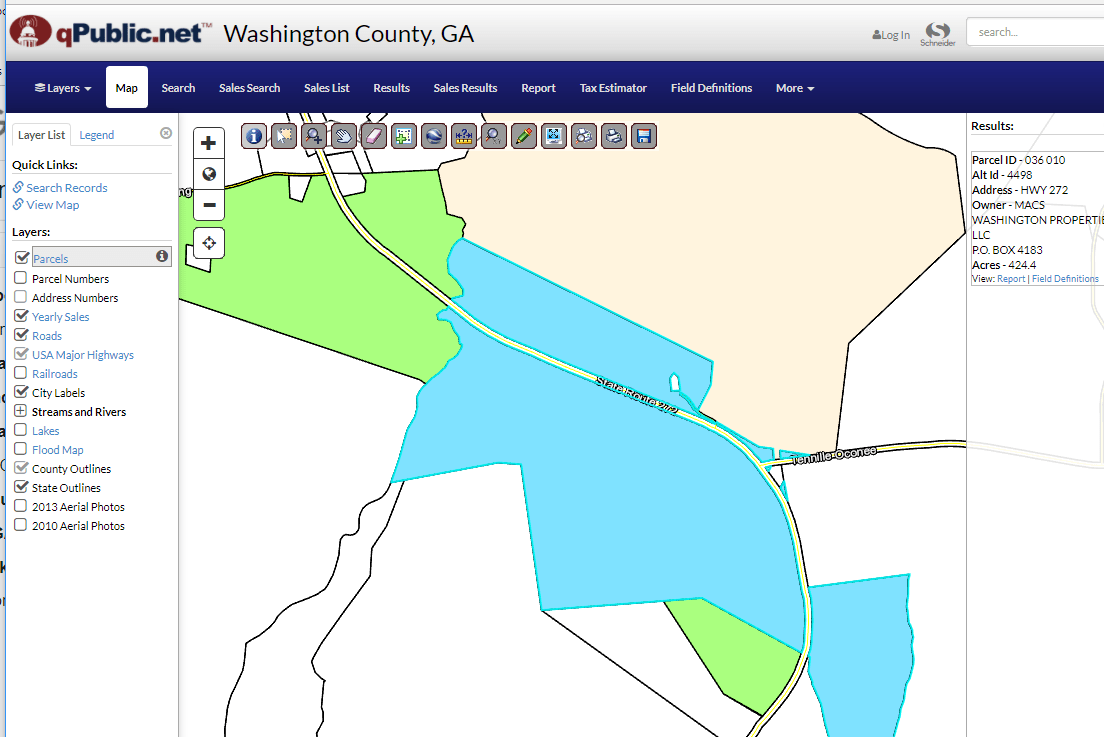
- Use the MAP tab to show the web-GIS
- The SEARCH tab takes you to monthly lists of Real Estate sales
- The SALES SEARCH tab takes you to a page where you can enter a custom query for Real Estate sales.
DOWNLOADing GOOGLE EARTH KML FROM QPUBLIC SITE
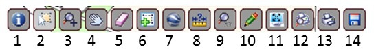
Locate the parcel of interest either by query (step 3 above) or by manually searching the GIS map (step 5 above). If you locate your parcel by manually searching the map, you need to zoom to your parcel and then use the select feature tool (tool #2 below) to select it.
While in the web GIS window (step 5 above), you will be presented with a list of selected parcels in the right-most part of the screen. If you want to view the property information the county has on file for this ownership, use the report link at the top of the screen. It never hurts to save this information in your working directory. You can save this page with a right-click > save as… You can also hit the print button and print to a PDF by changing the printer to PDF writer (you will most likely see something worded differently, but it will say PDF).
Once you are certain you have selected the correct parcel, use the Google Earth KML button (button #7) to save the KML boundary to your local machine.
Another word on file management!!!
If your web browser provides you an opportunity to specify where you want to save your file, then make sure you save it in your working directory. If your web browser, however, will probably automatically download to your Downloads folder. If and when this happens,
- Download the file
- Navigate to the Downloads folder using the File Explorer
- Copy the KML you downloaded to your working directory
- Recall that our working directory in labs 1 and 2 was c:\ocnatforest
————————————————————————————-
CONVERT KML TO FILE GEODATABASE FEATURE CLASS
————————————————————————————-
At this point, you should have a file with a KML extension in your working directory – use File Explorer to verify. The KML file is the native Google Earth format. You can not analyze a KML in ArcMap so you must first use the KML TO LAYER tool in ArcMap to convert from a KML to a file geodatabase feature class.
The KML TO LAYER tool is straight forward:
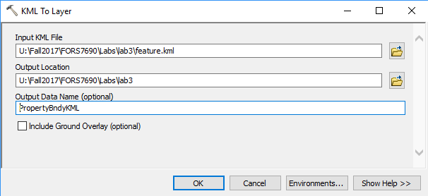
- Input …: Fully specify the path to your KML (use the file/open widget to do th)
- Output Location: Specify the path to your working directory (do not include the new file name)
- Output Data Name: Name of the file geodatabase that will be created in this process. The file geodatabase must not already exist.
This is what my working directory looks like in File Explorer before the KML TO LAYER process.

This is what my working directory looks in File Explorer like after the KML TO LAYER process.
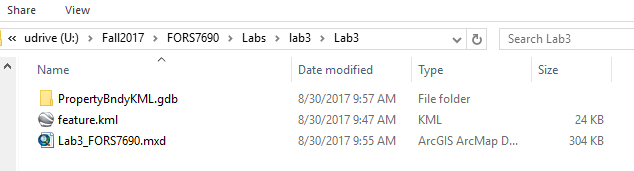
In the above example, the folder “PropertyBndyKML.gdb” is a file geodatabase (a folder within my working directory). Do not save anything inside this *.gdb folder.
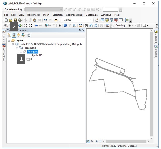
You will see a new layer in your ArcMap project after this process (screen shot below). Change the symbology to a dark outline and a hollow fill.
- This indicates that your feature class is a polygon layer.
- I am displaying the TOC by source. My feature class is saved in a file geodatabase called PropertyBndyKML.
Create file geodatabase and import layers
————————————————————————————-
ESRI’s file geodatabase (FGDB) is a more recent data standard in which the user may store vector (points, lines, polygons, raster, and tabular data. Run ArcMap’s CREATE FILE GDB tool to create your new FGDB.

Import layers into your new file geodatabase
————————————————————————————-
One of many ways to import GIS data into a FGDB is to use ArcMap’s FEATURE CLASS TO GEODATABASE command.
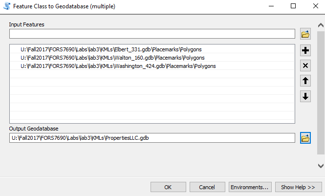
This import procedure creates three new feature classes in your PropertiesLLC FGDB. However, whenever possible, you want all of the polygons you plan to analyze stored in a single FGDB.
Merge feature classes into one feature class
————————————————————————————-
This procedure will put all of the polygons, I also call these features, from the three layers you created by running the Feature Class to Geodatabase command above into one feature class. Call this new feature class “PropertyBoundaries”.

————————————————————————————-
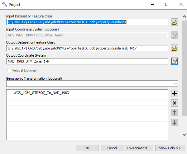
Project the PropertyBoundaries layer from Lat/Long coordinate system to UTM Zone 17, NAD1983 coordinate system
————————————————————————————-
Your data should be cast in a projected coordinate system any time you plan to make or report on area, perimeter, length, or any of the other possible geometries. The data from qPublic is cast in a Geographic coordinate system (Lat/Long). Use ArcMap’s PROJECT (DATA MANAGEMENT) command to mathematically transform your data to UTM coordinate space. In the Project dialog, you need to drill down and select (do not type) the Output Coordinate System NAD_1983_UTM_Zone_17N (hit the 4th button to browse the coordinate systems and drill down to Projected Coordinate Systems \ UTM \ NAD 1983 \ NAD 1983 UTM Zone 17N).
Prepare attribute table and calculate geometry
————————————————————————————-
Add two fields to your PropertyBoundariesUTM layer; one called “mytype” (text) and another called “gisacres” (float). Your attribute table should look like this:
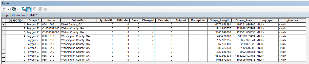
If you followed this approach to the letter, you have a field called “FolderPath” that contains the property’s county. This is an attribute carried over from the original KMLs. The other two fields of interest are “mytype” and “gisacres”.
Calculate acres.
If you are satisfied with your PropertyBoundariesUTM layer, remove all other layers in the TOC.
Verify that the layer is saved in your C:\ workspace (right-click on layer > Properties > Source Tab).
Save your project. Close your project.
Copy your working directory up to your network drive.
Wrap-up
————————————————————————————-
In practice, this entire process should take no more than 5 minutes.
We will continue work on this project during Monday’s digitizing lecture.