Spatial Analyst Toolset
Must load the Spatial Analyst extension to use these tools – Customize >> Extensions >> …
ESRI Spatial Analyst Toolset Listing
In last week’s lab, you used the following tools:
- Conditional – Raster If/Then operations
- Distance – When paired with a reclassification, this is how we buffer using the raster data type
- Extraction (specifically Extract by Mask) – Subsetting tools
- Map Algebra (specifically Raster Calculator) – Raster cell-by-cell operations
- Reclass (specifically Reclassify) – The means by which we change cell values
- Zonal (specifically Zonal Statistics as Table)
- Neighborhood (Block Statistics and Focal Statistics)
The scenario: Create an Ecological Geofence to assist with ‘green’ timberland track procurement.
You have been charged with assessing the company’s timberland holdings in Monroe Tennessee. Your task is to classify the landscape into three classes: 1) Acceptable, 2) Caution, 3) Not Acceptable – this will be our ‘Ecological Geofence’ layer. The decision criteria are listed below.
Data Layers: (Right-click > Save As on links below)
- Landcover – nlcd_tn_utm16.tif (UTM 16, NAD 1983)
- Rivers – nhd24kst_l_tn123 (UTM 16, NAD 1983)
- Streets – street100k_l_tn123 (UTM 16, NAD 1983)
- Protected Areas – clp_PADUS1_4 (UTM 17, NAD 1983): these are state and federally protected areas
- Elevation – MonroeTN_elev_cm.img (UTM 17, NAD 1983): elevation in centimeters
- Percent Slope – create from Elevation layer
All processing will be carried out using the UTM, Zone 17N, NAD 1983 coordinate system.
Decision Criteria:
- Bad Slope: Any area whose slope is greater than 20%
- BAD Protected Areas: All PAD designations
- BAD Landcover: Land_cover types: ‘Woody Wetlands’, ‘Emergent Herbaceous Wetlands’, ‘Open Water’, and any of the four Developed classes
- Bad Landcover: Any areas within 1000′ of ‘Open Water’
- BAD Streams: within 700′ of any stream with a GNIS_NAME and 300′ from all others
Set Working Environment
Geoprocessing > Environment Settings…
- Workspace > Current Workspace: c:\geofence\
- Workspace > Scratch Workspace: c:\geofence\
- Output Coordinates > Output Coordinate System: ‘Same as Layer “MonroeTN_elev_cm.img”‘
- Processing Extent > Extent: ‘Same as Layer “MonroeTN_elev_cm.img”‘
- Processing Extent > Snap Raster: MonroeTN_elev_cm.img
- Raster Analysis > Cell Size: ‘Same as Layer “MonroeTN_elev_cm.img”‘
Preliminary Data Processing
- Save your project into your working directory
- Reproject the three zone 16 data layers to zone 17
- Remove the zone 16 layers
- Save your project
Data Processing
SLOPE:
- Use the RASTER CALCULATOR to change the elevation units from centimeters to meters
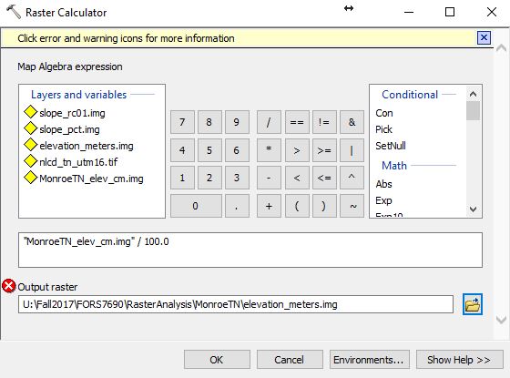
- Use the SLOPE command to create the slope layer
- make sure you use the elevation_meters.img layer as the input
- make sure you specify percent
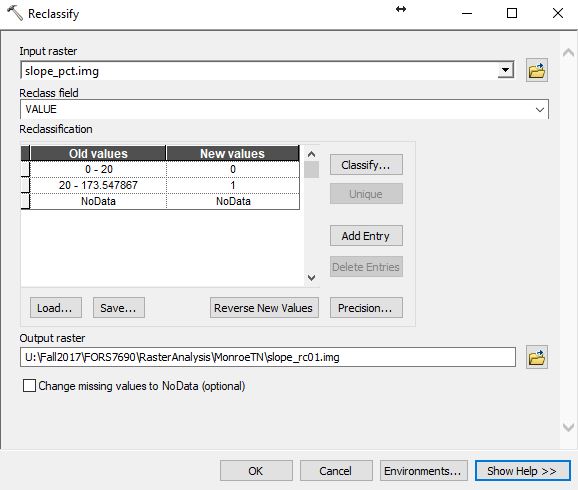
- Use the RECLASSIFY command to change values > 20 to 1 and everything else to 0
PROTECTED AREAS:
- Convert the vector Protected Areas layer to raster with the POLYGON TO RASTER tool
- Convert on the ‘Category’ field
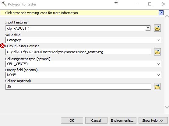
- Convert on the ‘Category’ field
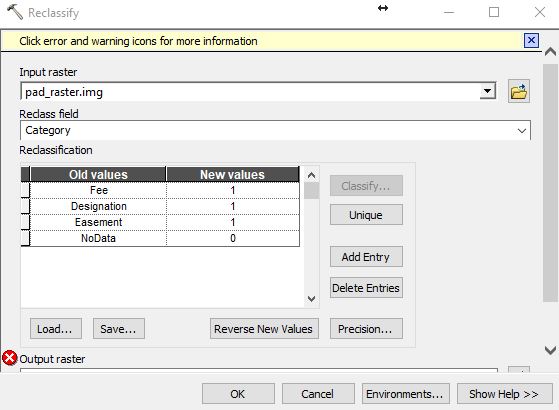
- Reclassify the pad_raster layer so all named cells have a value of 1 and everything else (NoData) has a value of 0
LANDCOVER:
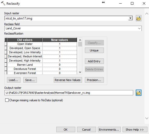
- RECLASSIFY the Landcover layer where ‘Open Water’, the four ‘Developed’ classes, ‘Woody Wetlands’, and ‘Emergent Herbaceous Wetlands’ are assigned a value of 1 and everything else a value of 0.
- Areas within 1000′ of Open Water
- RECLASSIFY the UTM 17 Landcover where water is given a value of 1 and everything else a value of zero
- Manually select the cells whose Value = 1 in the layer you just created
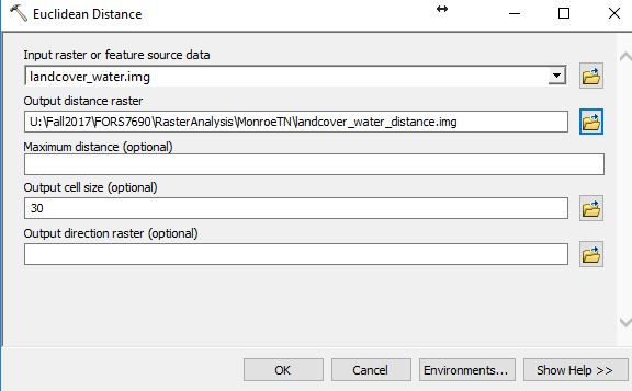
- Use the EUCLIDEAN DISTANCE command to generate a new layer whose Values reflect the straight line distance to the nearest water cell.
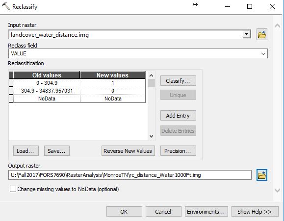
- Use the RECLASSIFY tool to change the Euclidean Distance values less than 1000 to 1 and everything else to 0
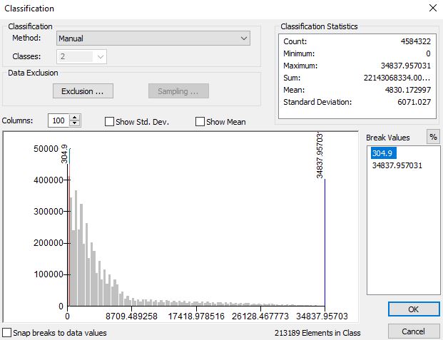
- Hit the Classify… button, change the Classes: value to 2, change the first break value to 304.9 (1000/3.28)
- Hit the Classify… button, change the Classes: value to 2, change the first break value to 304.9 (1000/3.28)
STREAMS:
- Convert the streams to raster with the POLYLINE TO RASTER; convert on the GNIS_NAME value field
- Process named streams:
- Manually select the records in the raster stream layer with a GNIS_NAME
- Run the EUCLIDEAN DISTANCE command
- RECLASSIFY all values < 213.4 (700′ / 3.28) to a value of 1 and everything else 0, give NoData a value of 0 too
- Process unnamed streams:
- Manually select the records in the raster stream layer with NO GNOS_NAME
- Run the EUCLIDEAN DISTANCE command
- RECLASSIFY all values < 91.5 (300′ / 3.28) to a value of 1 and everything else 0, give NoData a value of 0 too
COMBINE ALL LAYERS
- Use the RASTER CALCULATOR to combine all 1/0 layers
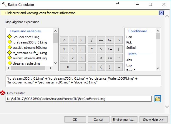
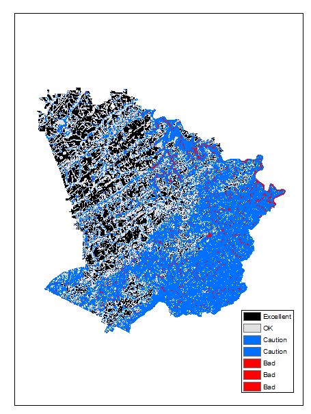
SUMMARY:
If you follow the workflow described above, you use a series of raster calculations, Euclidean distance measures, and reclassifications to generate a series of rasters whose values are either 0 or 1. A cell with a Value of 1 represents an area that satisfies the BAD criteria. The last step has the user combine these layers using addition. The result is a new raster layer with Values ranging from 0 to 5 where 0 are cells that do not meet any of the BAD criteria and 5 are cells that meet all 5 of the BAD criteria. However, you have no information about which BAD criteria are (or are not) met. Try the Spatial Analyst COMBINE command. I think it will produce the raster output we are looking for.