Seedling Survival Count from UAV – Demo

UAV-based Seedling Survival Count

Measuring Survival and Planting Quality in New Pine Plantations(Andrew J. and Stephen G. 2006)

BFGrant Demo Data (300MB) –

• download, copy the file to your C:\ workspace, right-click on the MXD > 7Zip > Extract Here, open the ../v105/Untitled.mxd ArcGIS project.
• figure out where the image is saved:  right-click on the ‘clp_bfg_south_DecemberORTHO_Low_2inPix.img’ layer > Properties > Source >…  The data folder is listed in the middle window under “File System Raster”.  Copy this path.
• Add Data > paste the path into the Add Data dialog > navigate into the ‘raster_data’ folder > … You will see the two raster layers that are already loaded in the project.
  • double-click on the ‘clp_bfg_south_DecemberORTHO_Low_2inPix.img’ image to reveal <Layer_1>, <Layer_2>, <Layer_3>
  • Select all three and hit ADD
• Save your project

The objective for today s for you to apply traditional ground-based seedling survival sampling methods to a UAV-based orthophoto.

Method #1: 1/100 acre circular plot (for BFGrant demo dataset)

The radius of a 1/100 acre plot is 11.775 feet, 3.58902 meters.  Traditional ground-based methods require the field worker(s) to 1) establish the radius, possibly by cutting a piece of string to length and staking it to the plot center, and then 2) counting the number of free-to-grow live, live-with-competition, and dead seedlings that fall within the plot.  A loose rule of thumb is 1 plot per acre.  Counts for each plot are recorded separately; your tally sheet might look like this:

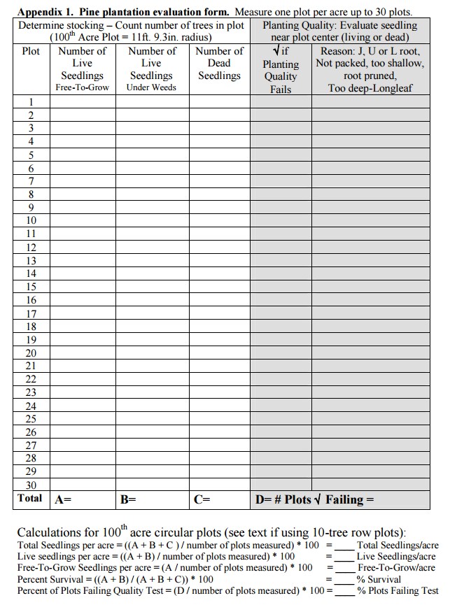
Manual seedling count from ortho

You could create your seedling survival sample point locations; generate the 11.775 foot buffer; manually count seedlings and record in the above tally sheet.

UAV-based census

Smoothing the Ortho

If there is too much noise in the image, you can smooth it out a little.  I ran a 5×5 and 10×10 focal mean (ArcToolbox>Spatial Analyst Tools>Neighborhood>Focal Statistics) across the clipped and UTM zone 17 projected image.  This step eliminates much of the noise (speckle) in the outputs I generate below.

Process Vegetation Index

In Raster Calculator:

GIndex.img =

Float( <Layer2> ) / Float ( <Layer1> + <Layer2> + <Layer3> )

GIndexCubed =

GIndex * GIndex * GIndex

Visually determine threshold that eliminates much of the non-pine noise.  Symbolize your vegetation index using Classified > Standard Deviation.  Pine have a higher value…

If you find a threshhold that you think works well, use the RECLASSIFY tool to classify the image into YES-PINE and NO-PINE.

Unsupervised (ISO) Classification

ArcToolbox>Multivariate>ISO Cluster Unsupervised Classification

• Input raster Bands: <Layer 1>, <Layer 2>, <Layer 3>
• Number of classes: 12

This did not look promising, I did not pursue this any further.

DEM-based processing

This one is difficult and required a little preprocessing.

• Buffer the rows by 0.5 meters
• Ran the Mean Shift (ArcToolbox>Spatial Analyst Tools>Segmentation and Classification>Segment Mean Shift) command to group similar, adjacent pixels
• Converted the layer to polygon (ArcToolbox>Conversion Tools>From Raster>Raster to Polygon)
• Next steps would be to
  1. run Zonal Statistics As Table using this Mean Shift layer as the zone layer and the GI or another spectral layer as the input raster
  2. filter based on the zonal statistic values