Monday, you had an opportunity to process a drone-based point cloud using R and the lidR and the rgdal packages. You should have familiarized yourself with the following commands and at least have an idea of what they do:
- plot()
- summary()
- lasfilterdecimate(): https://www.rdocumentation.org/packages/lidR/versions/2.0.0/topics/lasfilterdecimate
- lasground(): https://www.rdocumentation.org/packages/lidR/versions/2.0.0/topics/lasground
- lasnormalize(): https://www.rdocumentation.org/packages/lidR/versions/2.0.0/topics/lasnormalize
- lasfilter(): https://www.rdocumentation.org/packages/lidR/versions/2.0.0/topics/lasfilters
- grid_metrics(): https://www.rdocumentation.org/packages/lidR/versions/2.0.0/topics/grid_metrics
- grid_canopy(): https://www.rdocumentation.org/packages/lidR/versions/2.0.0/topics/grid_canopy
- writeRaster() – Make sure you provide a unique output name
- writeOGR() – Make sure you provide a unique output name
Let me point out a couple important steps in the code. Please see Monday’s lab for a full code listing and the lidR documentation for information about specific commands.
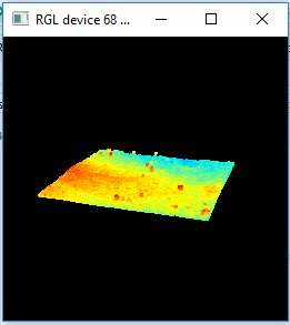
Use the plot() command to display an interactive plot of your LAS. Click-and-hold to rotate the plot and use the mouse wheel to zoom in and out.
plot(las)
Use the summary() command to list header information for your LAS.
summary(las)
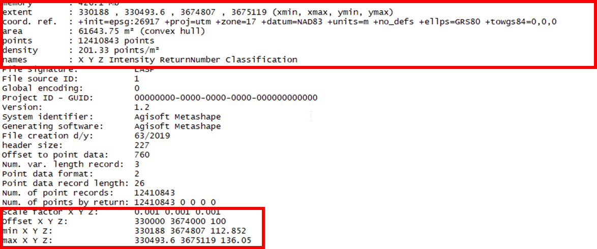
The original LAS file contains 12.4 million XYZ points – over 200 points/m2. That is a lot! The Z values range from 112.8 meters to a little more than 136 meters above sea level.
One approach to reduce the number of points is to employ the lasfilterdecimate() command. In lab, you used the random algorithm to reduce our density to 10 points/m2. Always use the summary() command to verify the process.
lasd<- lasfilterdecimate(las,random(10))
summary(lasd)
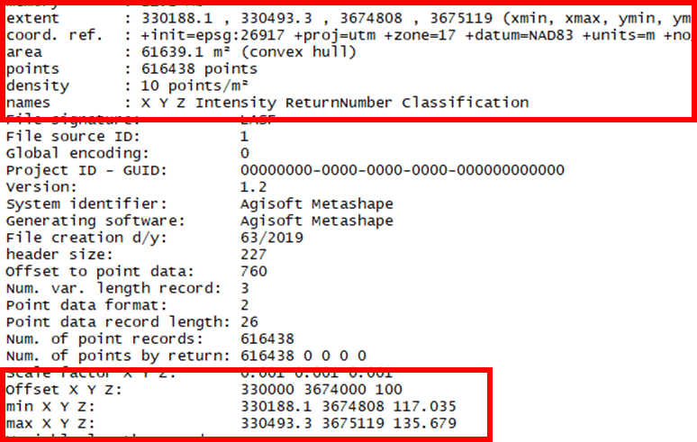
There are 616,438 points stored in my “lasd” object; 10 points/m2. The minimum elevation increased from 112.8 to 117. This is most likely due to the presence of “low noise”, points erroniously placed below the surface, in the original LAS. The maximum elevation decreased from 136.05 to 135.6. Also, notice I replace my “las” object with the decimated one I just created.
An important step in processing your point cloud data is to identify the ground surface. This will be the plane from which our height measurements are based. It is also the surface from which our “terrain model” will be generated and the surface you would use for your terrain analyses (slope, aspect, watershed, etc). You worked through two different approaches. The first approach had you use the lasground() command and the csf() algorithm. This approach is akin to draping a blanket across the bumpy surface. Parameters cloth_resolution, class_threshold, and rigidness control the analysis resolution, ground-cloth tolerance, and stiffness, respectively. The decision rule is any point below the cloth is classified as “ground”.
Next, you use this terrain model in the lasnormalize() command to remove the effects of terrain. The normalization process implemented in lab uses a KNN-based inverse-distance weighted approach to compute the “ground” level at each point. Normalization occurs when this value is subtracted from the current point’s elevation resulting in a “height above terrain” Z value instead of the original “height above sea level”. Afterwards, you should use the summary() command to view the maximum and minimum Z values.
summary(las_ground_normalized)

Notice that there are negative, -1.722m, and some rather high points, 11.032m, remining in the data. These points are removed using the lasfilter() command.
las_ground_normalized<- lasfilter(las_ground_normalized,(Z >= 0))
las_ground_normalized<- lasfilter(las_ground_normalized,(Z < 2))

The second terrain model creation command, grid_terrain(), uses a similar KNNIDW approach to find the ground surface. This time, however, the data is processed in raster-space.
Unlike the terrain model, the canopy height model, CHM, is a model of the surface that includes the terrain as well as all other objects present. The CHM result is raster, as well.
chm <- grid_canopy(las, res = 1, pitfree(c(0,2,5,10,15), c(0, 1.5)))
The lab finishes with a model of the individual tree crown apex points. You can fine-tune the model by adjusting the ws and hmin parameters.
ttops = tree_detection(las_ground_normalized, lmf(ws=2, hmin=1, shape = “circular”))