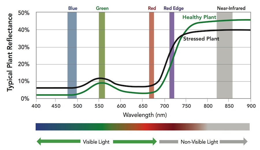
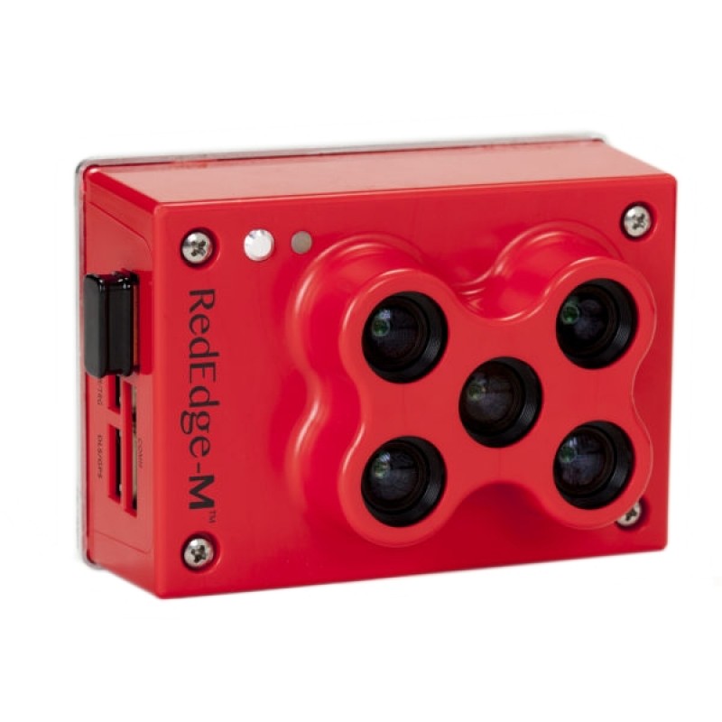
The MicaSense RedEdge-M a specialized sensor capable of recording reflected energy in the visible blue, green and red wavelengths as well as the non-visible red edge and near-infrared portions of the electromagnetic spectrum. Typical response of healthy plants, when compared to stressed plants, is lower in the visible and red edge wavelengths and higher in the near-infrared (figure below).
A typical workflow if you were interested in using this information to create a landcover classification, would be to:
- Perform a field visit where you record the “true” cover type and the plot location
- Fly the site with the multi-spectral camera
- Pre-process the multi-spectral imagery
- Convert the pixel values from the raw digital number (this is the pixel value stored when the image is captured) to percent reflectance (the amount of energy reflected off the object)
- Align the individual photos for each capture (see discussion below)
- Process the imagery in Agisoft, Global Mapper, or other photogrammetry software
- Generate any vegetation indices of interest (http://142.93.66.153/2017/04/24/vegetation-indices/)
- Sample the processed photos and vegetation indices at each field visit site
- You could use the EXTRACT VALUES TO POINTS, EXTRACT MULTI VALUES TO POINTS, or EXTRACT VALUES TO TABLE tools in ArcGIS to perform this task
- After this process, you have your ground-measured plot information associated with the blue, green, red, red edge, and near-infrared reflectance and any VI you create. (You have one record for each plot.) This is the table you will analyze.
- Run your analysis and analyze your results
- If you wanted to create a multi-layer image you can show in color, then use the ArcMap COMPOSITE BANDS tool…
- If your NDVI results are noisy, you could run a focal mean across the individual bands to smooth the inputs before compositing them
An issue with these multi-lens cameras is that each capture is comprised of, in the RedEdge-M case, five individual images. Each image is captured from a slightly different view (separate lenses) thus the resulting images are not exactly aligned.
This week in lab, you will step through a workflow where you 1) use the Fiji/ImageJ application to align the RedEdge-M photos, 2) transform the imagery into NDVI, and 3) sample the imagery at locations at which we have known, ground-measured information.
Please NOTE that these data are not georeferenced. You will be working in a generic, un-projected coordinate space. In this lab, ignore any Spatial Reference warnings you receive.
Download the lab data HERE.
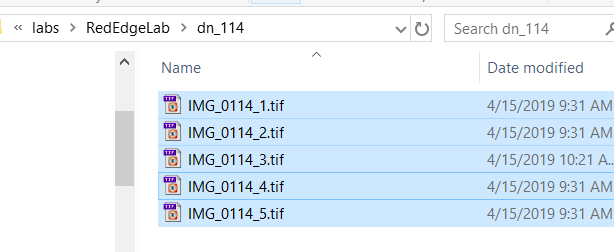
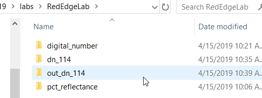
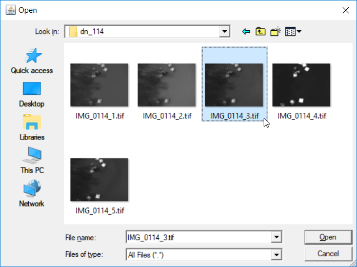
I have provided two image captures, image 0114 and image 0115, of the Moose-in-the-Lake statue out at Lake Herrick. An image capture consists of five individual images – one image for each band (blue, green, red, near-infrared, red edge). For example, the 0114 image capture is comprised of IMG_0114_1.tif, IMG_0114_2.tif, IMG_0114_3.tif, IMG_0114_4.tif, IMG_0114_5.tif. The raw, unprocessed image captures are stored in the “digital_number” folder. These are the images I transferred directly from the camera’s SD card. Their pixel values are not calibrated and are in the ‘digital number’ space and range from 0 to ~65500. I have also included the same images converted to percent reflectance – pixel values range from 0 to 1. There is a good discussion on the differences between DN and Reflectance HERE.
You will also use the Fiji/ImageJ app. Download the Windows 64-bit version HERE. This is a “green” application which means you do NOT install it like you would Word or other traditional software. All you need to do is unzip the software in your working directory and then run the Fiji.app\ImageJ-win64.exe file – no installation necessary.
The workflow I want you to follow for this lab is:
- Use the Fiji/ImageJ app to align each image capture stored in the digital_number and pct_reflectance directories
- Calculate NDVI for each image capture
- Compare the NDVI values at common points
- from each DN capture
- from each percent reflectance capture
- from each 0114 image
- from each 0115 image
Fiji/ImageJ:
You will be using the “Register Virtual Stack Slices” plugin (Plugins>Registration>Register Virtual Stack Slices) to align each image capture (ie bands 1 – 5 for image 0114; 0114_1, 0114_2, 0114_3, 0114_4, 0114_5). Your steps are:
- create a new folder for each image capture and copy the respective images over
- create folders dn_114, dn_115, refl_114, refl_115
- copy the image captures to the appropriate folder (5 individual images)
- create a new folder for each aligned image capture
- create folders out_dn_114, out_dn_115, out_refl_114, out_refl_115
- run the Register Virtual Stack Slices for each capture (see Screenshots below)
- Screen1: specify your input and output folders
- Screen2: select your reference image; this is the image to which the other images will be referenced
- Quit and restart Fiji to clear memory before processing the next image
- load the aligned photos into ArcMap for quality control and processing
Screenshots of Fiji/ImageJ workflow:
-

- Select your reference image
- new set of images in our output folder

Lab deliverable:
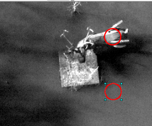
I want you to analyze two similar “Moose” spots and two similar “Water” spots across each image. Select two un-shadowed spots on the Moose’s back and two near by in the water. Make sure you can identify each location on all images you process in Fiji/ImageJ. Maybe these spots here…
Use the RASTER CALCULATOR to create an NDVI layer Float((band 4 – band 3) / (band 4 + band 3)) for each DN and reflectance image capture (dn_0114, dn_0115, refl_0114, refl_0115). Then, record the NDVI value at each of your four spots for each image capture. Since these images are not georeferenced, it is easier to use ArcMap’s Info button to query the pixel values (in a traditional workflow, you would overlay your point shapefile and run one of the commands I mention above to extract the pixel values). Your data sheet should look something like this:
| DN 114 – NDVI | DN 115 – NDVI | Refl 114 – NDVI | Refl 115 – NDVI | |
| Moose 1 | ||||
| Moose 2 | ||||
| Water 1 | ||||
| Water 2 |
Then, lets use the simple difference for our within-image NDVI comparisons
| DN 114 – NDVI | DN 115 – NDVI | Refl 114 – NDVI | Refl 115 – NDVI | |
| Delta Moose 1, 2 | ||||
| Delta Water 1, 2 |
Also use the simple difference for our between-image NDVI comparisons:
| Moose 1 | Moose 2 | Water 1 | Water 2 | |
| Delta DN 114, DN 115 | ||||
| Delta Refl 114, Refl 115 |
DeltaMoose1_2
NDVI ranges from -1 to 1.
I want you to compare…
within-image digital number (DN) and reflectance responses:
- Which within-image measurements are more similar, the DN Moose 1 and Moose 2 NDVI calculations or the Reflectance Moose 1 and Moose 2 NDVI calculations? (look at DN_114 Moose 1 and Moose 2, DN_115 Moose 1 and Moose 2, Refl_114 Moose 1 and Moose 2, Refl_115 Moose 1 and Moose 2)
- Which within-image measurements are more similar, the DN Water 1 and Water 2 NDVI calculations or the Reflectance Water 1 and Water 2 calculations? (similar comparison as above)
- Can you provide support from your data collection above to substantiate the following conclusion: Converting the pixel values to reflectance produced more stable NDVI measurements within each image… (Keep in mind that similar surfaces should yield similar NDVI values…)
between-image DN and reflectance responses:
- Are the image 114 and 115 Moose measurements more similar in the DN space or the reflectance space? DN114/Moose 1 vs DN115/Moose 1, Refl114/Moose 1 vs Refl115/Moose 1, …
- Are the image 114 and 115 Water measurements more similar in the DN space or the reflectance space?
- Can you provide support from your data collection above to substantiate the following conclusion: Converting pixel values to reflectance provided more stable NDVI measurements between image captures…
Record your results in a Word document and upload it to our ELC lab11 folder.