Lab 9 Data Link (clp_tls.laz). This is a large dataset, have patience!!! The “LAZ” file is a common point cloud file format storage type. You read a LAZ the same way you read a LAS – you process it using the same approach.
See the LAND USE, CARBON & EMISSION DATA (LUCID) portal, CIFOR and Wageningen University, to access another fascinating terrestrial LiDAR dataset that can be processed with this script as well (with minor changes).
Gonzalez de Tanago, J., Lau, A., Bartholomeus, H., Herold, M., Avitabile, V., Raumonen, P. Martius, C., Goodman, R. C., Disney, M., Manuri, S., Burt, A., Calders, K. (2017). Estimation of above-ground biomass of large tropical trees with Terrestrial LiDAR. Methods in Ecology and Evolution. DOI:10.1111/2041-210X.12904
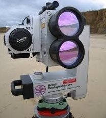
You will start with a point cloud from a ground-based LiDAR rig. This set up is also referred to as ”Terrestrial LiDAR”.
 ==>
==>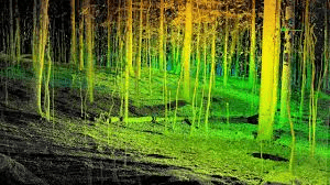
You are starting with a point cloud that looks like this:
 .
.
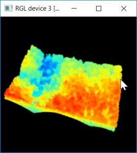
If you rotate the image up, you can see that this site consists of an upper, mature canopy with mid-story trees present in the openings. Researchers are interested in using this data to examine the individual trees. Your task is to segment the individual tree canopies and then calculate the min, max, and mean height (based on the point cloud) of each. Your segmentation will look something like this (where each color represents an individual tree crown): 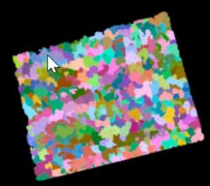
I’ve provided my code below…
#####https://www.rdocumentation.org/packages/lidR/versions/3.1.1
#####Dr. Tripp Lowe, Warnell School of Forestry and Natural Resources, UGA
#####
library("lidR")
library("rgdal")

#####Load Files
mypath<- "f:/uav/TerrestrialLiDAR_LLP"
myfile<- "clp_tls.laz"
infile<- file.path(mypath,myfile)
lastmp = readLAS(infile, select = "xyzirc")##, Intensity = F, ReturnNumber = F, NumberOfReturn = F, ScanAngle = F, EdgeOfFlightline = F, ScanDirectionFlag = F, UserData = F, PointSourceId = F, color = T)
summary(lastmp)
#####depreciated###lasd<- lasfilterdecimate(lastmp,random(250))  #lasdecimate
lasd<- decimate_points(lastmp,random(250))
plot(lasd)
summary(lasd)

#####Classify Ground Points.  This is used in the normalization process
#####depreciated###lasd<- lasground(lasd,csf(cloth_resolution = 0.5, class_threshold = 1, rigidness = 1), last_returns = FALSE)  ##classify_ground
lasd<- classify_ground(lasd, csf(cloth_resolution = 0.5, class_threshold = 1, rigidness = 1), last_returns = FALSE)
plot(lasd,color="Classification")

#####normalize, might take a little while to run
###depreciated###lasd_n<- lasnormalize(lasd, knnidw(k=10,p=2))  ##normalize_height
lasd_n<- normalize_height(lasd, knnidw(k=10, p=2))
plot(lasd_n,color="Classification")
summary(lasd_n)
lasd_n<- filter_poi(lasd_n,(Z >= 0))
plot(lasd_n)
summary(lasd_n)
lasd_nbak<- lasd_n

#####create terrain and surface model
col<- pastel.colors(250)
#####dtm1 = terrain model "bare ground model"
dtm1<-grid_terrain(lasd_n, res = 0.5, algorithm = knnidw(k=25,p = 0.5))
plot(dtm1)

#####chm = surface model
chm<- grid_canopy(lasd_n, res=0.5,p2r(0.3))
plot(chm)
ker <- matrix(1,3,3)
chm <- raster::focal(chm, w = ker, fun = mean, na.rm = TRUE)
plot(chm)

#####detect individual tree tops and crowns
###depreciated###ttops <- tree_detection(chm, lmf(4, 2))  ##find_trees
ttops<- find_trees(chm,lmf(4, 2))
##depreciated##lasd_n<- lastrees(lasd_n,mcwatershed(chm,ttops))
lasd_n<- segment_trees(lasd_n,dalponte2016(chm, ttops))
###deprecited###crowns<- watershed(chm)()
crowns<- dalponte2016(chm, ttops)()

plot(crowns)
x = plot(lasd_n, color = "treeID", colorPalette = col)
add_treetops3d(x, ttops)

#####Export DTM, DSM, Crowns, and tree tops; view these in ArcMap. They do not have a
#####defined coordinate system but the data are to scale; meters are the unit of measure.
dtmOut<- "TerrainModel.tif"
chmOut<- "CanopyHeightModel.tif"
crnOut<- "TreeCrowns.tif"
ttopOut<- "TreeTops"
writeRaster(dtm1 ,filename = file.path(mypath,dtmOut), format="GTiff",overwrite=TRUE)
writeRaster(chm, file.path(mypath,chmOut), format="GTiff",overwrite=TRUE)
writeRaster(crowns, file.path(mypath,crnOut), format="GTiff",overwrite=TRUE)
writeOGR(obj=ttops,dsn=mypath, layer=ttopOut, driver="ESRI Shapefile", overwrite=TRUE)


#####Generate statistics for each tree;  Trees were identified with the "lastrees(lasd_n,mcwatershed(chm,ttops))" command
myMetrics = function(z, zr)
{
  metrics = list(
    zmean = mean(z),
    zmax  = max(z),
    zmin  = min(z),
    zrmean = mean(zr),
    zrmax  = max(zr),
    zrmin  = min(zr)
  )

  return(metrics)
}
treestats<- tree_metrics(lasd_n, myMetrics(Z, Zref))
metricsOut<- "TreeMetrics.csv"
write.csv(treestats, file= file.path(mypath,metricsOut))


#####Statistics for groups of trees @ 30ft (30/3.28)m, 60ft (60/3.28)m, 90ft (90/3.28)m
#####First create filtered copies of the lasd_n point cloud
lasd_n30ft<- filter_poi(lasd_n,(Z <= (30/3.28)))  ###filter_poi
lasd_n60ft<- filter_poi(lasd_n,((Z > (30/3.28)) & (Z <= (60/3.28)))) ###filter_poi
lasd_n90ft<- filter_poi(lasd_n,(Z > (90/3.28))) ###filter_poi
plot(lasd_n30ft, color="treeID", colorPalette = col)
plot(lasd_n60ft, color="treeID", colorPalette = col)
plot(lasd_n90ft, color="treeID", colorPalette = col)
####output 30ft stats
treestats30ft<-tree_metrics(lasd_n30ft, myMetrics(Z, Zref))
csvoutname<- "TreeMetrics_30ft.csv"
write.csv(treestats30ft, file = file.path(mypath, csvoutname))
####output 60ft stats
treestats60ft<-tree_metrics(lasd_n60ft, myMetrics(Z, Zref))
csvoutname<- "TreeMetrics_60ft.csv"
write.csv(treestats60ft, file = file.path(mypath, csvoutname))
####output 90ft stats
treestats90ft<-tree_metrics(lasd_n90ft, myMetrics(Z, Zref))
csvoutname<- "TreeMetrics_90ft.csv"
write.csv(treestats90ft, file = file.path(mypath, csvoutname))
At this point, you have exported several raster TIFs and a point shapefile that you can view in ArcMap. You will get a Spatial Reference warning since these data do not have a defined coordinate system. This is one of the few instances where you can ignore this warning.
TerrainModel.tif: This is the ground model (DTM). It was generated using the normalized point cloud, so its values should be near 0.
CanopyHeightModel.tif: This is the surface model, the DSM. This layer was generated using the normalized point cloud, so its values reflect the pixel’s height above the (TerrainModel) surface. The units of measure are meters.
TreeCrowns.tif: This raster layer contains the individual tree crown segmentation. It was created with the following command:
segment_trees(lasd_n,dalponte2016(chm, ttops))
The raster values are the sequential number assigned to each individual tree crown. This layer is exported as a float raster, so before you convert it to a polygon layer, you must run the INT(Spatial Analyst) tool in ArcMap to convert the real numbers to integers. Convert that output to a polygon layer with the RASTER TO POLYGON, and then join the CSV summaries on the gridcode and treeID fields.
TreeTops.shp: This is a point shapefile marking each crown’s apex.