UAV-Mapper output (orthophoto, surface model, LAS) from the first part are stored in your working directory in a folder named “5_Products”. For this lab, however, use the point cloud I provide in the data you downloaded at the beginning of part 1:
"clpSG_PointCloud_th001.las"
which is saved in the “PhotoscanOutput” folder in the data packet. The data is saved on my computer on the U:\ drive on the FANR5640\Spring2021\Week08\Nov30_2017a\PhotoscanOutput\ path. Thus, my working directory is:
U:\FANR5640\Spring2021\Week08\Nov30_2017a\PhotoscanOutput
Use the File Explorer to locate your working directory – it will be different than mine.
IN THE FOLLOWING, I STEP YOU THROUGH A LiDAR WORKFLOW TO SEGMENT THE TREE CANOPIES…
The first few lines of code load the necessary R libraries and defines my working directory and input file names. We will leverage point cloud functionality provided by the lidR library. We will be using version 3.1.1 of the lidR library(rdocumentation and https://rdrr.io/cran/lidR/) and the most recent versions of raster and sp. If you are curious about its use and common workflows, see this Remote Sensing of Environment article.
Remember that you must change the inpath variable to match your working directory. Also, you must use either forward slashes (/) or double-back slashes (\\) when specifying your working directory.
#####https://rdrr.io/cran/lidR/
#####install libraries if not already
#####install.packages("lidR")
#####install.packages("raster")
#####install.packages("sp")
library(lidR)
library(raster)
library(sp)
library(rgdal)
myfile<- "clpSG_PointCloud_th001.las"
inpath<- "U:/FANR5640/Spring2021/Week08/Nov30_2017a/PhotoscanOutput"

#####create folder for outputs
outfolder<- "outputs"
if (file.exists(file.path(inpath,outfolder))){
} else {
  dir.create(file.path(inpath,outfolder))
}
outpath<- file.path(inpath,outfolder)

mylas<- readLAS(file.path(inpath,myfile))
We report the LAS header information on line 6. Pay attention to the
- coord. ref.: the defined coordinate system
- area: planar area of the data in units of the coordinate system
- points: # points in the LAS
- density: points per square unit
- min X Y Z: minimum values
- max X Y Z: maximum values
summary(mylas)
Plot the point cloud and look for outliers. Click-and-hold the left mouse button to rotate; right-click-and-hold to pan; scroll in/out to pan in/out.
plot(mylas)
You will next classify the ground points using the classify_ground method. I present the CSF method for its speedy processing. This step sets each point’s “Classification” attribute to either 0 (never classified) or 2 (ground). The classification values are listed in Table 4.9 of the ASPRS LAS Specification document.
lasgrnd<- classify_ground(mylas, csf(
              sloop_smooth = FALSE,
              class_threshold = 0.5,
              cloth_resolution = 0.5,
              rigidness = 3))
plot(lasgrnd, color = "Classification")

max(lasgrnd$Classification)
min(lasgrnd$Classification)
hist(lasgrnd$Classification)
hist(lasgrnd$Z)
Now that we have the ground points classified, we can use the grid_terrain method to generate the digital terrain model. In the code below, I analyze each point in context of its 10 nearest neighbors (knnidw algorithm). I finish this section of code off by saving the raster DTM out as a new file to the output directory I set up at the start.
outdtm<- "myDTM.tif"
dtm<- grid_terrain(lasgrnd,res = 0.5, algorithm = knnidw(k=10, p=2), keep_lowest = TRUE)
plot(dtm)
writeRaster(dtm,filename=file.path(outpath,outdtm), overwrite=TRUE)
Use the grid_canopy command to create and export the digital surface model (DSM).
outdsm<- "myDSM.tif"
dsm<- grid_canopy(lasgrnd, res=0.5, algorithm=pitfree(c(0,2,5,10,15), c(0, 1.5)))
writeRaster(dsm, filename=file.path(outpath,outdsm), overwrite=TRUE)
At this point in the code, our point cloud is still reporting the Z attribute in terms of mean sea level. Lets normalize the point cloud so Z reflect height above the ground surface. There are several methods associated with the normalize_height method, but I am using the expedient knnidw again. Some of the points end up with a below-zero normalized height; you can see this when you look at the min Z values. Use filter_poi to remove these points. You could also use the summary() command.
lasnorm<- normalize_height(lasgrnd, knnidw(k=10, p=2))
max(lasnorm$Z)
min(lasnorm$Z)

#####filter points less than 0
lasnorm<- filter_poi(lasnorm, !(lasnorm$Z < 0))
max(lasnorm$Z)
min(lasnorm$Z)
plot(lasnorm, color = "Z")
A canopy height model (CHM) is a raster layer whose pixel values reflect an object’s height above the ground surface. Use the grid_canopy command to rasterize the normalized point cloud. (We used this command above to create the DSM, but we input the un-normalized point cloud.) I also run a 3-pixel by 3-pixel focal mean across the CHM twice to remove some of the remaining pits or holes in the canopy.
chm <- grid_canopy(lasnorm, res = 0.5, pitfree(c(0,2,5,10,15), c(0, 1.5)))
plot(chm)

kernel<- matrix(1,3,3)
chm3a = raster::focal(chm, w=kernel, fun=mean)
chm3a = raster::focal(chm, w=kernel, fun=mean)
plot(chm3a)
Now that we have our CHM, lets find the trees with the find_trees command. This section attempts to find the apex, those tree tips, across the landscape.
ttops<- find_trees(lasnorm,lmf(ws=1, hmin = 0.15))
plot(ttops)
x=plot(lasnorm)
add_treetops3d(x,ttops)
Now, based on each tree top, segment each unique tree with the segment_trees command and delineate each crown with delineate_crowns and write them out to a shapefile.
crowns<- segment_trees(lasnorm,dalponte2016(chm3a,ttops,th_tree=0.15))
plot(crowns, color="treeID")

hulls<- delineate_crowns(crowns, func = ~list(Zmean = mean(Z)))
writeOGR(hulls,dsn=inpath,layer="hulls2", driver="ESRI Shapefile")
At this point, you have generated two raster layers, the DSM and DTM, and a polygon layer representing each tree crown (“hulls2” in the last line of code). Load these and the orthophoto I provide and compare. How well are the tree crowns delineated? According to my initial test (figure below), not too well.
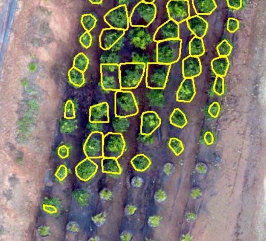
We need to find places in our code to improve. More on that later… Save your work.