Georeferencing Scanned Maps

Georeferencing scanned maps

The data you have been working with so far has been prepared for somewhat easy incorporation into ArcMap. Data scientists from the NRCS Geospatial Data Gateway carefully processed the aerials you used in last week’s lab; ensuring all of the roads, rivers, buildings, etc. were in their proper geographic location. If these data were not in their proper location, any other GIS data would not align when overlain in ArcMap.

The NRCS NAIP aerials have been processed to a strict standard. The photos are acquired on a cloud-free day and during the growing season for (mainly) crop insurance purposes. After transfer to the computer, adjacent photos are color-balanced and stitched together. The photos are then assigned their ‘proper ground location’ through a process called orthorectification. Orthorectification is the process of removing the effects of image perspective (tilt) and relief (terrain) effects for the purpose of creating a planimetrically correct image. The resultant orthorectified image has a constant scale wherein features are represented in their ‘true’ positions. This NAIP technical report has a pretty good explanation of their plane-to-product processing steps.

Consider the road running from the northeast to the southwest shown in the photos below. The road in the photo on the left appears to be crooked. This displacement is due to the uneven terrain. Scale throughout this image is not constant – shape, area, and distance are distorted in this unprocessed image. “Non-costant scale” implies that the area represented on the ground by 1-square inch in one part of the photo does not equal the area represented by the same 1-square inch in another part of the photo. This is a problem especially if your plan it to make management decisions based on measurements from this photo.

In reality, the road is straight as seen in the photo on the right. Inputs for the orthorectification process are a series of well-located and easily recognized ground control points (GCP) and a digital elevation model (DEM). A well-defined ground control point is a distinct location one can recognize in the field and on the photo. Examples of suitable GCPs are sidewalk corners, road intersections and other street markers, driveway corners/edges, and any other easily recognized low-to-the-ground objects. Examples of unsiutable GCPs are edges of a roof or the top of a building or the top of any tall object, meandering curves of a river or timber cutline, and any feature that might move (ie. cars). The DEM is a raster layer whose pixel values represent elevation.

orthorectification

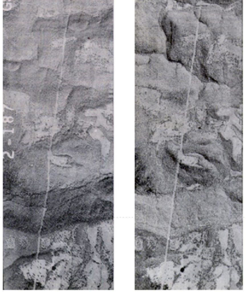
The above two images are of the same geographic area.  Note the road that passes through the mountains.  In the left "raw" or unrectified image, the road appears to be crooked when in fact is is not.  The image on the right has been rectified and the road appears planimetrically correct. (https://trac.osgeo.org/ossim/wiki/orthorectification)

Rubber sheeting

ESRI Fundamentals of georeferencing a raster dataset

OCFP SAMPLE DATA

We will be applying a simpler method of correcting our un-georeferenced photos called rubber-sheeting that does not require a DEM to align two layers. You will use the Geoprocessing toolbar in ArcMap to stretch an un-georeferenced image across a NAIP image. The processing steps are something like this:

load a base map “source” image that has a properly defined coordinate system – NAIP imagery are suitable
ensure your data frame coordinate system is set correctly to match the NAIP (View > Dataframe Properties > Coordinate System tab)
load your un-georeferenced “target” image (in our case, the Dan Williams scan)
load the Geoprocessing toolbar
locate and click on the first GCP in the target image
locate and click on the exact same location in the base image
repeat three more times then check RMSE (Georeferencing toolbar > View Link Table button)
…
update your georeferencing or resample to new image

Root-mean-square-error (RMSE)

ArcMap reports forward RMSE in the unit of your data frame coordinate system. The inverse residual reports RMSE in terms of ‘number of pixels’. If you are using UTM, then RMSE units are meters, if you are using State Plane, then the RMSE units are feet. If your data frame coordinate system is using the WGS84 geographic projection, then your RMSE will be in decimal degrees – this is an extremely bad idea (using a geographic-projected layer as the source, that is)!

Rule-of-thumbs (for this class):  1) RMSE should be less than or equal to 1/2 the side dimension, in map units, of a pixel.  The NAIP imagery, for the most part, have a 1-meter pixel, therefore your RMSE shold be .le. 0.5 meters.  2) Additionally, the georeferenced image must pass visual inspection.  If there are areas of misalignment, you need to add, remove, or adjust GCPs.

The goal here is to stretch the scanned image across the georeferenced image so they align, not to generate a low RMSE.  You can generate a solution with a low RMSE and have poor alignment!

RMSE: “A measure of the difference between locations that are known and locations that have been interpolated or digitized.” (ESRI)

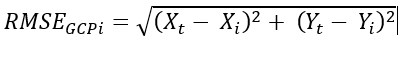rmsegcpi_lowe2 , where X_t and Yt are the transformed coordinates and X_i and Y_i are the source (ground-measured) coordinates and RMSE_GCPi are the squared residuals for each point. (NOTE: ArcMap recalculates the transformed coordinates each time you add a new GCP.) This is the distance in ground units between the transformed coordinates of the point you clicked in the target image and the coordinates of the point you clicked in the source image.

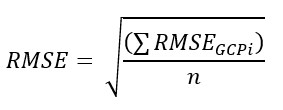rmsetotal_lowe2 , where RMSE_GCPiare the individual squared residuals you calculated above, n is the number of GCPs you inserted, and RMSE is the square root of the mean squared residuals.

Since in statistical terminology, we typically use a small number of GCPs, refrain from assigning a meaning to RMSE. Instead, use the total RMSE as a guide to how well you have done overall and the individual RMSEs to locate possible egregious mistakes. When working on small parcels like Lake Herrick, the best indication is a visual inspection.

National map accuracy standards (NMAS)

NMAS define the accuracy standards for published maps, including horizontal and vertical accuracy, accuracy testing method, accuracy labeling on published maps, labeling when a map is an enlargement of another map, and basic information for map construction as to latitude and longitude boundaries.

In a nutshell:

at scales larger than 1:20,000, not more than 10% of the points tested shall be in error by more than 1/30th of an inch (measured at the publication scale),
- 0.033333 x RF scale x 2.54 / 100 = error tolerance in ground meters
at scales 1:20,000 and smaller, not more than 10% of the points tested shall be in error by more than 1/50th of an inch (measured at the publication scale)
- 0.02 x RF scale x 2.54 / 100 = error tolerance in ground meters

These NMAS calculations should be performed on an independent dataset – the points you use in these calculations should NOT be used in the georeferencing process.

Example:

If you publish a map with a scale of 1:15840, no more than 10% of the points tested shall be in error by more than