FANR3800: Overlay Analysis I (Topological Overlays)

Overlay Analysis

We have already reviewed one overlay (selection) analysis tool – Select By Location. Recall, with this method, you select whole records in one layer that are spatially related in some manner (intersects, within a distance…, center is within…, etc) to another layer (Select By Location). This method works well if you need to know “which or how many whole features in the CoverType layer are intersected by any of the features in the Streams layer?” or “what or how many whole line segments are within 50’of one of the nesting sites?” or any of the thousands of questions relating to “What is on top of what”. However, since Select By Location selects whole features, you are NOT able to answer the “how much area is within the 50′ buffer?” or “how many linear feet of our interior road system are within a SMZ?” or the thousands of other questions relating to “HOW MUCH” with this approach.

Topological analysis techniques

(ESRI Online Help Doc)

The following topological analysis techniques produce a new output layer that

are some combination of 2 or more existing layers that MUST be cast in the same coordinate systems,
if there are any selected features in any of the inputs, are some combination of only those selected features,
contain new features (buffer) or existing features whose shape has been changed in some way (intersect, erase, union, etc), therefore you must recalculate geometry every time you run one of these commands,
retain the attributes from either one or all of the inputs

Topological analysis operations (clip, erase, update, union, intersect)

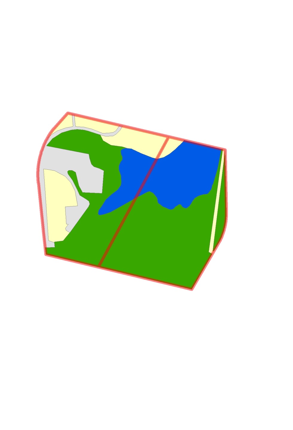
The following examples show the results of various topological overlays of the ‘input’ and ‘overlay’ layers shown below. The input layer is a polygon landcover with the CoverType, Acres, and abbr attributes. The overlay layer is a proposed sale boundary with two polygons and the following attributes: Acres, SaleArea, UnitPrice, and Owner.

INPUT: 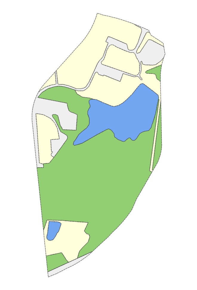$U:\Fall2015\FANR3800\lecture\Wk6\CoverType.jpg$

OVERLAY: 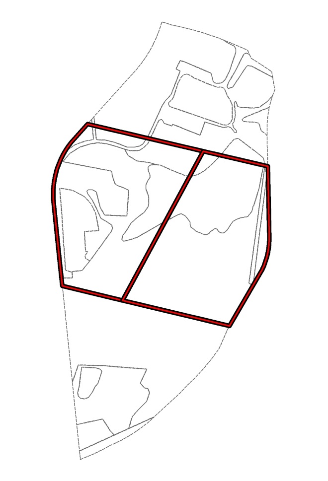$U:\Fall2015\FANR3800\lecture\Wk6\SaleArea.jpg$

The clip command

ArcToolbox > Analysis Tools > Extract > Clip

$U:\Fall2015\FANR3800\lecture\Wk6\clip.jpg$

This is the cookie-cutter operation. This operation retains the area within the overlay layer.
Output only contains the attribute information from the input layer
Acreage is not automatically updated so you MUST recalculate the area geometry.

The erase command

ArcToolbox > Analysis Tools > Overlay > Erase

$U:\Fall2015\FANR3800\lecture\Wk6\erase.jpg$

This command removes the area within the overlay data layer.
Output only contains the attribute information from the input layer
Acreage is not automatically updated so you MUST recalculate the area geometry.

The update command

ArcToolbox > Analysis Tools > Overlay > Update

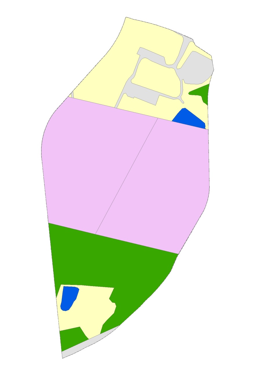
$U:\Fall2015\FANR3800\lecture\Wk6\Update.jpg$

This command replaces the areas in the input layer with the shapes in the overlay layer.
- The original input is colorized by the CoverType field attributes (field, water, forested, hard surface). The purple updated areas do not have one of these attributes so the new polygons fall into that ‘all other values’ category which is symbolized with a purple fill.
Output only contains attributes from the input layer
Acreage is not automatically updated so you MUST recalculate the area geometry.

The union command

ArcToolbox > Analysis Tools > Overlay > Union

$U:\Fall2015\FANR3800\lecture\Wk6\SaleUnion.jpg$ $U:\Fall2015\FANR3800\lecture\Wk6\SaleUnion2.jpg$

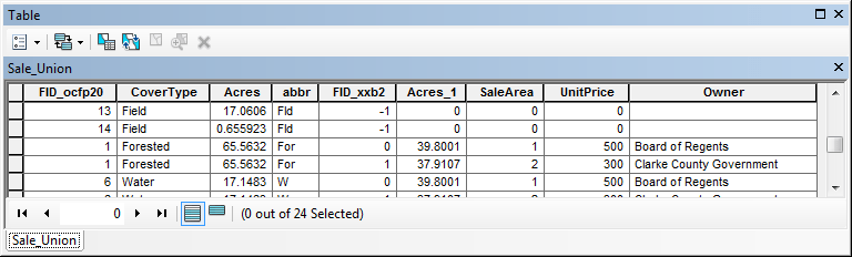
This command burns in the polygon boundary of the overlay layer into the shapes of the input layer
- Extent of new data layer is the union (all) of the areas
Output contains attributes from both input and overlay layers
Make note of the FID_xxb2 field (-1 means the polygon was not created by the overlay polygon)
Acreage is not automatically updated so you MUST recalculate the area geometry.

The intersect command

ArcToolbox > Analysis Tools > Overlay > Intersect

$U:\Fall2015\FANR3800\lecture\Wk6\SaleIntersect.jpg$ $U:\Fall2015\FANR3800\lecture\Wk6\SaleIntersect2.jpg$

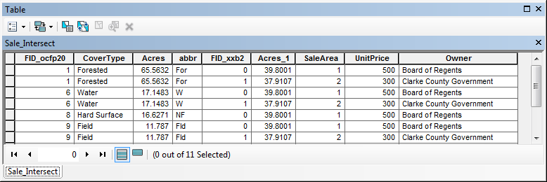
This command burns in the polygon boundary of the overlay layer into the shapes of the input layer
- Extent of new data layer is the intersection of the areas Only the areas where both layers overlap
Output only contains attributes from both input and overlay layer
Acreage is not automatically updated so you MUST recalculate the area geometry.

Topological operators summary (Primarily, how much area)…

Clip, Erase, Update, Union, Intersect
Results in changes in a feature’s shape and, in some cases, additions to a layer’s attribute table (see last Wednesday’s lecture)
Why is it called a topological operation?
- Involves rebuilding the topological relationships that facilitate spatial analysis
- Topology means “What is next to what”Which polygons are next to which? Which lines run into which lines? Etc…
  - Vector topology is explicit – it is created by the user
- New lines and polygons are formed from various possible combinations
- The new features inherit attribute data from one or both of the original datasets

Quick Review of Attribute and Spatial Queries (How many records satisfy)…

Every feature in a layer has attribute data
Relational operators: >, <, =, <=, >=, <>
Boolean operators: And, Or, Not
- AND: both criteria must be true
- OR: at least one criteria must be true
Follow parenthesis rules…
Selection methods
- Create New
- Add To
- Select From
Spatial Selections: Select features from layer based on their spatial relationship with another layer
- The spatial selection in the example below, “select all polygons that are intersected by the red polygon”, will select all 6 whole polygons.
The attribute and the spatial queries operate at the record-level – only records and their related (whole) shapes are selected

Associated Methods…

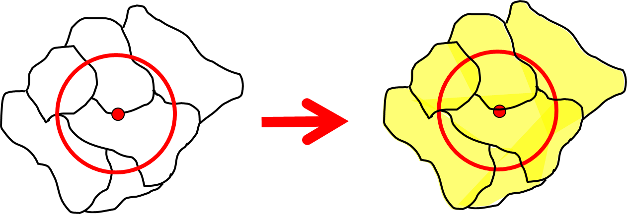
Buffer

Geoprocessing pull-down >> Buffer or ArcToolbox >> Analysis Tools >> Proximity >> Buffer

Can be applied to points, lines, and polygons
Always results in a new polygons layer
The user specifies a buffer distance and buffer units
A negative buffer distance yields a buffer inside the polygon

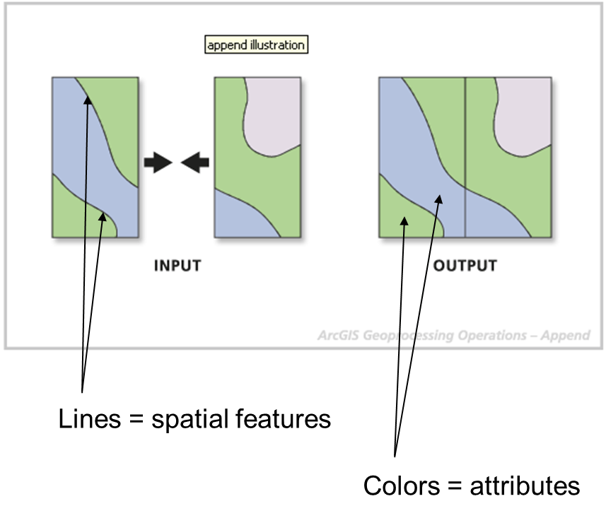
Append

Arctoolbox >> Data Management Tools >> General >> Append

Used to combine spatially-adjacent data layers

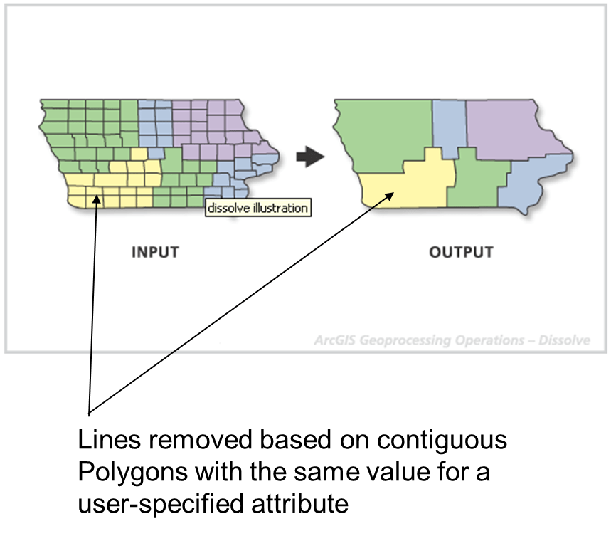
Dissolve

Arctoolbox >> Data Management Tools >> Generalization >> Dissolve

Merges a layer’s polygons or lines
- Merge may be based on an attribute (for instance county or state name)
Many times, after appending layers, you will end up with arcs where the layers are joined
These arbitrary boundaries can cause problems
- Require additional data storage
- Increase processing time
- Will bias analyses based on feature area or perimeter

Multipart To Singlepart (Explode)

Arctoolbox >> Data Management Tools >> Features >> Multipart To Singlepart

Many times, operations such as the dissolve command result in multipart features. A multipart feature is a geographic object that is made up of non-contiguous features (points, lines, or polygons) but is considered as one record (has only 1 record) by the software. For example, the state of Hawaii could be considered a multipart feature because its separate geographic parts are classified as a single state. Visually, this layer would appear to have many polygons. However, it would only have one record in the attribute table.

The multipart to singlepart command explodes these multipart features into singlepart features.

Putting it all together…

To actually do a spatial analysis, we typically need to use multiple spatial operations, for example

Append two stand layers that cover your study area
Clip the appended layer down to the landscape you want to analyze
Buffer a stream layer to create a new streamside management zone (SMZ) layer
Intersect the buffer layer with the stand layer to create a new layer with stand and SMZ information
Query the combined layer to get information on the total area, total timber volume, and distribution of forest types within the buffers

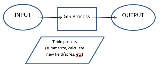
Before performing a spatial analysis, you must:

understand the question(s) being asked, and
be able to break the task into multiple parts

Break the analysis up into input > process > output and repeat if necessary.

spatialdiagram1

Examples

How many acres of each landcover type do we spare if we can’t harvest within 200’ of a river?

… harvest within… implies you must buffer
… acres of each landcover type do we spare… implies we are interested in the area outside of the buffer region… could use the erase command
… How many acres of each landcover… implies we must summarize type by summing acres