Download the following three compressed files and unzip them (preferably to a new folder you create on the C:\ drive).
Whitehall Dam Photos (Download Link)
My Whitehall Dam ReCap Photo w/out GCP Output (Download Link)
My Whitehall Dam ReCap Photo with GCP output (Download Link)
Stack Profile Line Shapefile (Download Link)
Last lab you generated a 3D model of the Warnell woodpile using Autodesk ReCap Photo. The source photos for that project did not contain any geo-location information, thus the model output was not georeferenced, nor was it scaled correctly. Recall that you had to assign a scale to the model based on the orange ruler before you were able to generate realistic volume measurements.
In this lab, you will process a set of photos that are geotagged. The geotag information is stored in each photo’s EXIF tags in the form of a latitude, longitude, and altitude. Use Windows Explorer to navigate to one of the photos, then (right-click > Properties > Details tab); scroll down to the GPS section. You will see coordinate information similar to this: 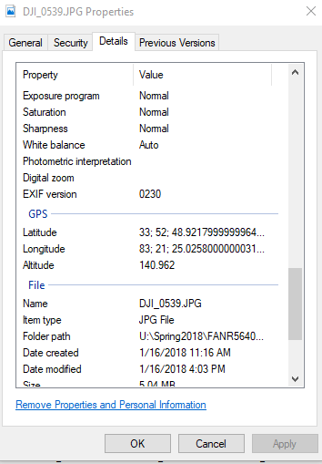
Make note that the GPS coordinates are presented as Lat/Long in Degree/Minute/Second (DMS) format. Also, you need to remember that Altitude is measured in meters above sea level (ASL). As a rule-of-thumb, the error in GPS altitude is 3 to 4-times larger than the horizontal error.
In today’s lab, you will process the Whitehall Dam photoset using two different workflows – one without GCPs and one with GCPs. The output from the first workflow will not be georeferenced – further geoprocessing is required to get it GIS-ready. The output from the second workflow is georeferenced and suitable for immediate geographic analysis.
Process 1 – Geotagged photos w/out GCPs
Unzip the Whitehall Dam Photos data (linked at the top of the page)
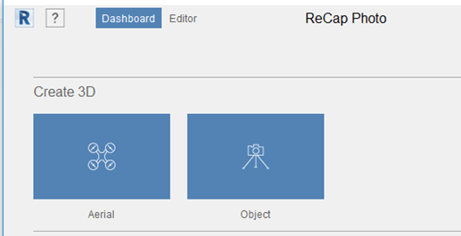
- Sign into ReCap Photo
- Create an Aerial mission
- Upload your photos
- Hit Create
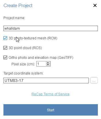
- Name your project, tick the point cloud and ortho buttons
- ReCap Photo tries to select the appropriate coordinate system based on the EXIF tags. Either UTM84-17 or UTM83-17 will work
- Hit Start, Wait
- You will receive an email from Autodesk when the processing is complete. At that point, you can download the project from your Autodesk cloud space or directly from the ReCap Photo interface.


Process 2 – Geotagged photos with GCPs
Now process the same photo dataset using ground control points. The steps for this are similar to processing w/out GCPs. You will:
- Upload your UAV photos to Autodesk ReCap Photo
- Insert your ground control points (GCPs)
- Specify ‘3D point cloud and Ortho photo and elevation map (GeoTIFF)’ in the Create Project dialog
- Hit Start and wait for the job to finish processing
A ground control point is a point with a known geographic location (X, Y, Z) that is easily found on the ground and easily seen in the photos. In photogrammetry, GCPs are used to register a photograph to known X, Y, and Z location – this process is referred to as georeferencing. In an ideal situation, the UAV operator would lay out targets throughout the study area and record their locations with a high-accuracy GPS. However, any stable distinguishable feature can serve as a GCP (shiny rock, end of a parking space line, manhole cover). I did not lay out GCP targets for this mission so you will have to use other GCPs (small rocks, a hard edge, a foot print in sand, the northwest corner of my equipment case, etc). The GCP UTM/NAD1983/Zone17N coordinate information (GCP Number, UTM X, UTM Y, Altitude in meters) is:
1, 282523.903364, 3751068.96883, 163.0
2, 282545.771741, 3751077.772140, 160.18
3, 282551.970649, 3751089.440380, 163.51
4, 282505.774836, 3751094.91192, 161.28
5, 282546.149998, 3751088.828700, 159.89
6, 282570.229575, 3751067.22372,160.70
Your task is to locate each of these GCPs (see image below – full resolution image here) on at least four individual photos. 
Start the process by opening ReCap Photo and creating a new Aerial project – do not hit the Create button yet. This is the point in the process where you locate your GCPs. Open the GCP window  , paste the comma-separated list (from above) into the GCP window, set the Coordinate System to UTM83-17. You should see something like below.

Insert GCP 1:
GCP 1 is a corner on the dam. Click on GCP 1 in the GCP Window and then click on the same spot in at least four photos. This spot is easy to find, look on photos 0007, 0015, 0020, 0100, 0151 and numerous other photos.
When you click on your first photo, the cursor changes to a cross-hair and the mouse wheel lets you zoom in and out. Zoom in close to your target and click on the corner of the dam. When you are satisfied with the marker’s location, hit Done. 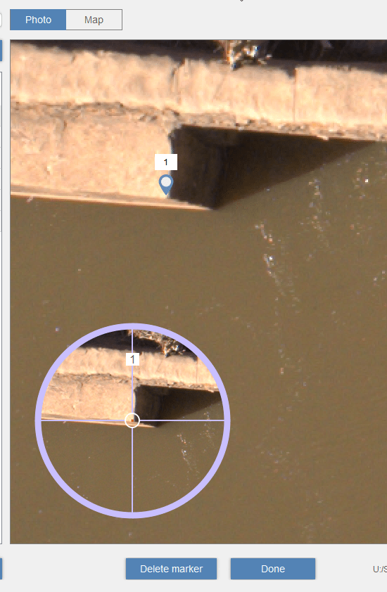
If you are sitting at a screen that looks like the screenshot below, click on the blue box that says “Place GCPs on at least 3 more images”. 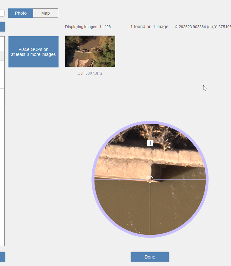
It might also help to untick the “Filter by GPS” box when you see it at the top of the page. Once you have inserted at least 4 GCPs, select the next entry in the GCP list and repeat.
Insert GCP 2:
GCP 2 is triangle-shaped rock on the northern side of the delow-dam sandbar

Insert GCP 3:
GCP 3 is the top corner of the down-stream retaining wall (north of GCP2 and east of GCP5)

Insert GCP 4:
GCP 4 is a patch of weeds above the dam on the northern side of the river.

Insert GCP 5:
GCP 5 is a white rock west of GCP 3, at river level on the northern side of the river.
Insert GCP 6:
GCP 6 is a little white rock down-river of the sand bar. Look for a stick in the water. 
The orange exclamation circle will turn green when you have inserted enough GCPs. Once you have placed all 6, hit the blue Done button (screenshot below) to upload to Autodesk server and begin processing.

View my processing results:
You will receive an email from Autodesk announcing that your job is finished processing and is ready to download. Follow the link they provide to your A360 cloud space and download your project. Instead of waiting for your jobs to finish processing, lets take a look at the with and without GCP projects I submitted last week.
You should have already downloaded the with and w/out GCP projects linked at the top of the page. Uncompress the Whall_Dam_YesGCP and WhallDam_NoGCP files (right-click > 7Zip > Extract Here). Your project files you download from A360 also contain the original photos you processed; I have deleted them from these zip files to save space and download time.
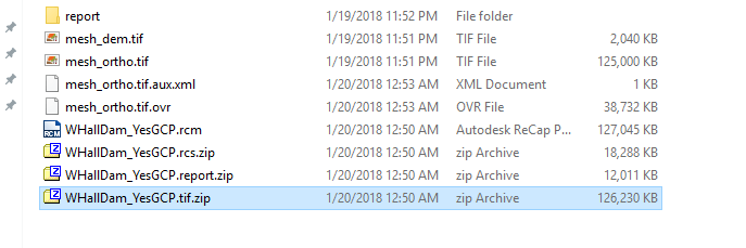
After unzipping, drill down into the ‘..YesGCP’ folder and unzip WHallDam_YesGCP.tif.zip and WHallDam_YesGCP.tif.zip (right-click > 7Zip > Extract here). Your file structure will look like the screen shot below. Make note of these file’s path, you will use it in just a minute.
The report (report.html) contains minimal information about the orthophoto generation. Give it a look, you will see similar reports from other software.
In ArcMap:
Load the ..YesGCP mesh_dem.tif and mesh_ortho.tif images in a new instance of ArcMap.
File > Add Data > Add Data; navigate to your data path and select both images then hit Add
Make note of the coordinates shown in the lower-right corner – those are lat/long values even though you specified UTM in the ReCap Photo workflow.
Now load the ..NoGCP mesh_dem.tif and mesh_ortho.tif images. Zoom to the NoGCP ortho (right-click on the layer > Zoom to Layer). Make note of the coordinates shown at the bottom of the page. The NoGCP layers are not georeferenced!
Zoom back to the YesGCP layers and remove the NoGCP layer.
Symbolize the dem:
Right-click on the dem layer > Properties > Symbology tab > …
- Select “Classified” on the left
- Click the Classification button and select Quantile > Hit OK > Hit Apply
Create a stack Profile:
Load the 3D Analyst tool: Customize pull-down-menu > Extensions > tick the 3D Analyst box
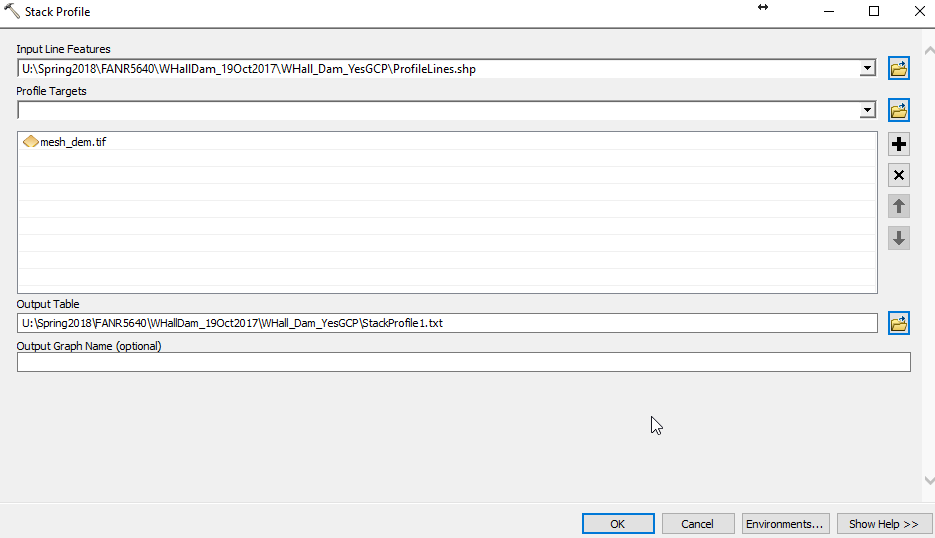
Use the ArcGIS Search tool (Windows pull-down-menu > Search) to find the “Stack Profile (3D Analyst) tool.
- Input Line Feature: ProfileLines shapefile (download at the top of the page, you must unzip the file you download)
- Profile Target: the …YesGCP_dem layer
- Output Table: navigate to the folder you set up for this lab and call the output “StackProfile.txt”
- Open Excel and drag the StackProfile.txt file onto the Excel canvas.
- Select the first column > Data tab > Text to Columns
- Delimited, hit Next
- Comma, hit Finish
Your Excel worksheet should look like this
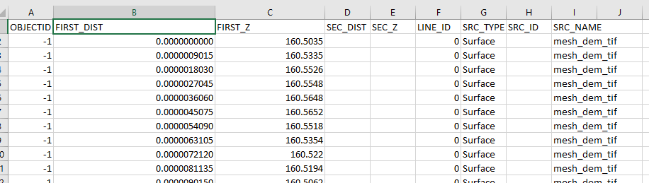
Note that the distances are in decimal degrees since all of our data in ArcGIS are in a geographic (Lat/Long) coordinate system. We should have first projected all of our inputs to UTM/NAD83/Zone 17N/Meters before we ran the stack profile tool, but for this exercise, we’ll deal with DD.
Select the data in the FIRST_DIST and FIRST_X columns and insert a scatter plot. Your profile will look something like this:
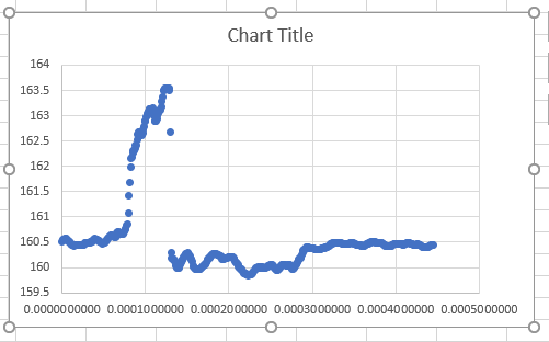
My example is not pretty, but you can clearly see the elevation change from above and below the dam.
For your first lab homework assignment, upload your stack profile chart to the lab 2 ELC dropbox. Try to make yours prettier than mine!