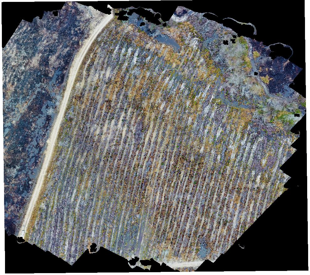
The data you are looking at are from a flight on December 14, 2016 in south Georgia. ‘P4_SouthGA_14Dec16_ORTHO02.img’ is the Agisoft 3-band, 0.02 meter resplution, natural-color orthophoto output. ‘P4_SouthGA,14Dec16_DEM08’ is the Agisoft 0.08 meter resolution terrain model generated from the same data.
Set up your project workspace
- Download the data files that arelinked at the top of the page.
- Open File Explorer and create a new folder on the C:\ drive called Lab3
- Copy the zipped file (probably in your Downloads folder) over to the C:\Lab3 folder
- Right-click on the zipped file (make sure it is the one in the C:\Lab3 folder) >> Extract All
- Repeat for lab data 2
- Open ArcMap
- Open the Catalog (Windows >> Catalog)
- Click on the folder-with-a-plus-sign icon (third icon from the left along the top of the Catalog window)
- Select the C:\ drive in the Connect To Folder dialog that appears (this reveals the entire C:\ drive to ArcGIS)
- Save your project as ImageClassification in the C:\Lab3 folder
- Environmental Settings (Geoprocessing pull-down menu >> Environment Settings)
- Current Workspace: C:\Lab3
- Scratch Workspace: C:\Lab3
- Since you will be doing image classification, you need to make sure the Spatial Analyst extension is loaded (Customize pull-down menu >> Extensions >> tick the box next to Spatial Analyst)
- Periodically, <CTRL-S> to save your project
- Open the Catalog (Windows >> Catalog)
Load multi-layer image vs. Load individual bands
KEY DISTINCTION – Add a multi-layer image vs Add a single layer of a multi-layer image
- File > Add Data > Add Data
- When you navigate to the folder in which you saved your image, you will see something similar to the screen capture below:
- You will LOAD the multi-band, color orthophoto if you click once on the layer and then hit Add.
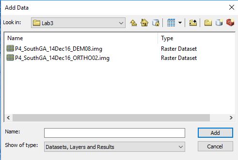
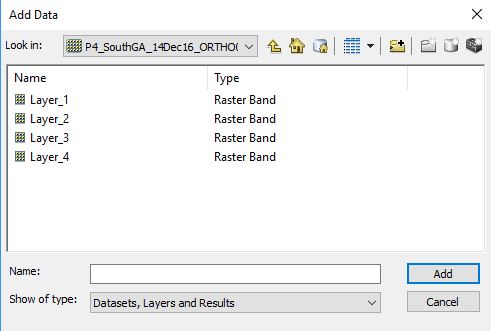
- Alternatively, if you double click on the P4…ORTHO, you will see the individual layers in the image. This is how you load the individual layers of a multispectral image (you will do this in just a minute).
- You will see a grayscale image if you load one of these
Do not let me proceed with the lab until you internalize this difference!!! Questions?
Right-click (on layer) >> Properties…
The steps below only change the way the image appears on the screen.
Change raster color combinations (the Symbology tab)
Natural Color
- Red: Layer_1
- Green: Layer_2
- Blue: Layer_3
Change the image’s appearance
- Stretch Type: ESRI or Standard Deviations are the best
- Statistics: Change the extent from which the stretch statistics are generated
Project the raster from UTM, 17N, NAD 1983 (HARN) to UTM, 17N, NAD 1983
NOTE: You can view the projection properties, if they are defined, under the Properties >> Source tab
Use the Project Raster command
Open the Search window (Windows pull-down >> Search)search for ‘project raster’you are looking for ‘Project Raster (Data Management)’
Use the following entries in the Project Raster dialogInput Raster: P4_SouthGA_14Dec16_DEM08.imgOutput Raster Dataset: E:\Lab3\P4_SouthGA_14Dec16_DEM08_u17N.imgOutput Coordinate System: use the projection dialog to Scroll down to ‘Projected Coordinate Systems’ folder >> UTM >> NAD 1983 >> select NAD_1983_UTM_Zone_17NHit OK
Repeat for the orthophoto
Reset the View’s coordinate system
View pull-down menu >> Data Frame Properties >> Coordinate System tabScroll down to ‘Projected Coordinate Systems’ folder >> UTM >> NAD 1983 >> select NAD_1983_UTM_Zone_17N<CTRL-S>
Clip images to stand boundary
Load the StandBoundary shapefile to the view if you have not already.
- Search for Extract by Mask (Spatial Analyst)
- Input raster: …DEM08.img
- Input raster or feature mask data: StandBoundary
- Output raster: clp_dem08.img (use the file/open dialog to ensure the output is placed in the C:\Lab3 folder)
- Repeat using the …ORTHO02.img layer as input. Call this one clp_ortho02.img
Band combinations (vegetation indices)
Our image data today:
- Blue: Layer_1
- Green: Layer_2
- Red: Layer_3
List of vegetation indices: http://www.harrisgeospatial.com/docs/BroadbandGreenness.html
We have access to Blue, Green, and Red information, so without the NIR layer, we are somewhat limited in terms of published VIs. For instance, the VARI index formula is
VARI = (Green – RED) / (Green + Red – Blue),
and in terms of our image
VARI = (Layer_2 – Layer_3) / (Layer_2 + Layer_3 – Layer_1)
Here is another list of vegetation indices: https://www.aeroeye.com.au/industries/agriculture/multispectral-imagery-and-vegetation-indices/
Personally, I have had success with
GI = (Green) / (Blue + Green + Red)
Compute a vegetation index (GI)
- Load the individual ortho bands (Layer_1, Layer_2, and Layer_3)
- These will appear as greyscale images
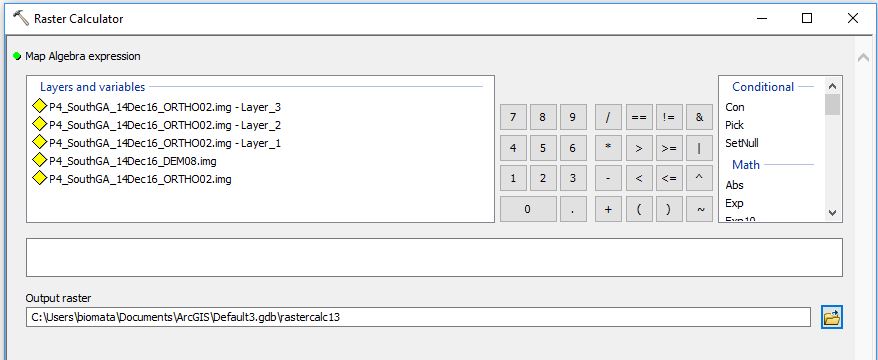
- Open the Raster Calculator (search for it in the Search window)
- If you get an error message, you have not loaded the Spatial Analyst extension (instructions near the top of the page)
- If you get an error message, you have not loaded the Spatial Analyst extension (instructions near the top of the page)
- The formula will look like this:
- Float(<<Layer_2>>) / Float(<<Layer_1>> + <<Layer_2>> + <<Layer_3>>)
- Compute the GI, with cursor in the middle box:
- type Float
- click ‘(
- double-click on Layer_2
- click ‘)’
- click ‘/’
- type Float
- click ‘(‘
- double-click on Layer_1
- click ‘+’
- double-click on Layer_2
- click ‘+’
- double-click on Layer_3
- click ‘)’
- Name your output c:\Lab3\GI.img (notice the .img extension)
- Try to calculate the Green Leaf Index, Normalised Green Red Difference Index, Vegetation AR Index Green, and Vegetation Index Green (from https://www.aeroeye.com.au/industries/agriculture/multispectral-imagery-and-vegetation-indices/). Make sure you name the outputs with a .img and that you save them in the E:\Lab3 folder.
Unsupervised image classification in ArcGIS
Intro video: https://www.youtube.com/watch?v=l5eHogds9zQ
Follow the Unsupervised Image Classification tutorial to classify the ORTHO. DEM, and your vegetation indices.
To turn in to lab 4 dropbox
Present in a Word document:
- The vegetation index formula and a screen shot that produces an image that appears to best discriminate among pine seedlings and everything else
- An explanation why using an unsupervised classification is not the best analysis approach for the terrain model.