Download the “Lab6Data” file HERE (you can also find the Lab6Data.zip file in our FANR5640_7640 folder on the N:\ Drive). Use File Explorer (type Explorer in the search window in the lower-left of the screen) to copy the zipped file you just downloaded (look in the Downloads folder) over to a new file you create on the c:\ drive (navigate to the C:\ drive>right-click>New Folder). Unzip the data file in this new folder.
- Turn off Background Processing in ArcMap (Geoprocessing menu>Geoprocessing Options>untick Enable under Background Processing)
- Load the Spatial Analyst extension in ArcMap (Customize menu>Extensions>Check the box next to Spatial Analyst)
- Save your project to the folder you create on the C:\ drive
- Load all of the images in the Lab6_BFG_03Dec2017_1_3cm.gdb file geodatabase (lots of them)
Segment Mean Shift
Image Segmentation is the process of identifying (and grouping) adjacent pixels with similar spectral characteristics. ArcGIS implements this process through the Segment Mean Shift routine where the user controls the amount of spectral detail, the amount of spatial detail, and the minimum segment size in pixels. Image output will contain 1..n unique classes. Furthermore, if your input image is a multi-layer raster, your output will be a multi-layer raster.
- spectral detail: Set the level of importance given to the spectral differences of features in your imagery. Valid values range from 1.0 to 20.0. A higher value is appropriate when you have features you want to classify separately but have somewhat similar spectral characteristics. Smaller values create spectrally smoother outputs. For example, with higher spectral detail in a forested scene, you will be able to have greater discrimination between the different tree species.
- spatial detail: Set the level of importance given to the proximity between features in your imagery. Valid values range from 1.0 to 20. A higher value is appropriate for a scene where your features of interest are small and clustered together. Smaller values create spatially smoother outputs. For example, in an urban scene, you could classify an impervious surface using a smaller spatial detail, or you could classify buildings and roads as separate classes using a higher spatial detail.
- minimum segment size: Merge segments smaller than this size with their best fitting neighbor segment. Units are in pixels.
I processed our BF Grant image with spectral detail 1, 5, 10, 15, and 20 across spatial detail 1, 5, 10, 15, and 20 using the ArcPy script at the end of this document (figures 1 and 2). Notice in Figure 1 how the pine seedling detail decreases as the spectral detail decreases. The top-left pane demonstrates ESRI’s statement that a higher value is appropriate when you have features what to classify separately but have somewhat similar spectral characteristics. The effect of changing the spatial detail is seen in Figure 2. The output image retains many small unique clusters when the user sets the spatial detail to 20, but only the most unique clusters are retained when the spatial detail is set to 1.
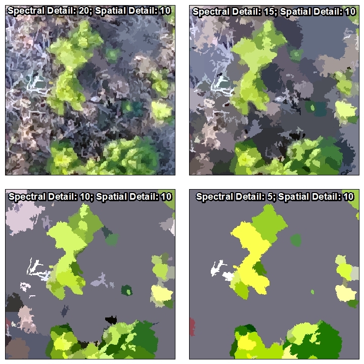
Figure . Changing spectral detail parameter
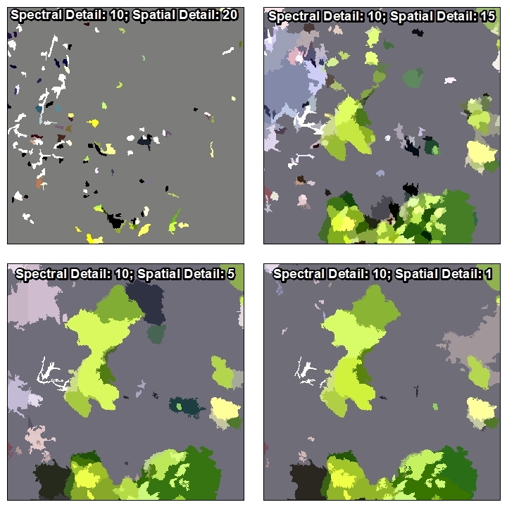
Figure . Changing spatial detail parameter
Workflow for this lab
- Select “best” segmented image and run the Compute Segment Attributes (tool)
- Select “suitable” signature polygons and process signatures
- Run the Train Maximum Likelihood Classifyer (tool)
- Run the Classify Raster (tool)
- Evaluate your classification
Select the “best” segmented image
Think back to last week when you performed a supervised classification. You drew a polygon around homogenous features and then assigned an attribute. These polygons, in practice, should be around 100 pixels in size and as homogenous as you can make them. This week, instead of drawing the polygons you will select one of the segmented images and use a subset of its segments to create your image classification training set.
By visually comparing the segmented images with the original RGB image, I selected the spectral detail = 15, spatial detail = 10 image. I think this image is a good balance between segment size and detail. You, on the other hand, might find another segmented image suits your needs.
I will use the ‘BFG_03Dec2017_15_10’ image as my source for training samples.
Select suitable signature polygons and process signatures
Recall from last week that your training signatures need to be labeled. In this step, we will attempt to select a group of segments for our “pine”, “coarse woody degris”, “brown plant”, and “other” classes.
- Load the Image Classification toolbar (right-click in the grey ArcMap banner>select Image Classification)
- Your image target (set in the Image Classification toolbar) should be the segmented image you determined to be the best in the steps above
- Activate the ‘Select Segment’ tool instead of the ‘Draw Polygon’ tool

- Open the Training Sample Manager (icon to the right of the target image window)
- Collect your PINE signatures one-by-one
- Zoom into a pine seedling and double-click on it
- Enter the class name in the signature editor
- Repeat for COARSE WOODY DEBRIS “CWD”
- Repeat for low-lying green “LLG”
- Repeat for any other class you are interested in
- Once you have selected all of your training sites, use the ‘merge signature’ tool on the Training Sample Manager

- Select all of your pine signatures in the Training Sample Manager dialog and hit the merge signatures
- Repeat for your other classes
- Save the signatures out as a file (hit the diskette in the Training Sample Manager and save it out as a shapefile called “TrainingSignatures.shp” in your working directory and outside of your file geodatabase)
- Save your project
Run the TRAIN MAXIMUM LIKELIHOOD CLASSIFYER tool
- Input is the original image
- TrainingSignatures.shp is your input training file
- Output classifier definition file should be saved outside the file geodatabase, call it “TrainingSignatures_Definition”
- Incluce your segmented image in the Additional Input Raster
- I selected segment attributes too

Run the CLASSIFY RASTER tool
- Input is your RGB image
- Input Classifier Definition File: TrainingSignatures_Definition.ecd (from above)
- Output: save it in your file geodatabase
- Additional Input Raster: your ‘best’ segmented image

Evaluate your classification
Upon visual comparison, I see my initial classification of PINE and BROWN is terrible, but the CWD appears to capture some of the larger material. 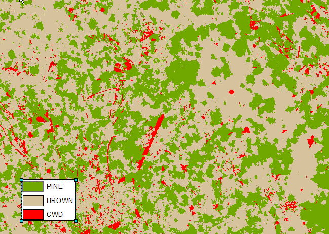
Look at MY classification (above and below this line) that included the segmented image with a classification that does not include the segmented image in the CLASSIFY RASTER routine.
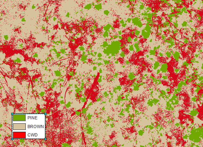
My classified image is pretty bad. I need to go back to the Training Sample Manager and refine my signatures and run the process again. My PINE class was over-classified. To address this, I will 1) evaluate my PINE signatures – did I include non-pine areas my mistake?, and 2) I will include more samples of the objects that “were classified as pine but are actualy something else.” I think I might also reconsider my best segmented image.
TURN IN FOR THIS LAB
I want you to use the above approach to classify the original RGB image twice. Your classifications should be based on the segmented image you consider the ‘best’ for our purposes (discrimination of pine, cwd, brown plants, low-green plants, …). Colorize the classes (green for pine, brown for brown plants, red for CWD, …) and paste a screen-shot in a Word document and describe where the classification failed.
Next, go back to the Training Sample Manager and refine your classes making sure you address the mis-classifications you mention above. It might be easier to create a completely new set of signatures instead of editing the existing signatures you have already created. Insert a screenshot of this new classification, colorize it the same way, and describe if your attempts to refine the classification yielded a better classification; are there areas where the 2nd classification is not as good as the first.
Upload your Word document to the Lab 6- Object-Based Classification assignment ELC dropbox.
ArcPy script to generate the Segment Mean Shift images:
import arcpy, os
from arcpy.sa import *
arcpy.CheckOutExtension("Spatial") ##load spatial analysis extension
specDetailstr = ["01", "05", "10", "15", "20"]
spatDetailstr = ["01", "05", "10", "15", "20"]
workPath = "u:\\Spring2018\\FANR5640\\Segmentation\\BFG_03Dec2017_1_3cm.gdb\\"
imageName = (workPath + "BFG_03Dec2017_1_3cm")
print imageName
minSegSize = 20
     for specDet in specDetailstr:
          for spatDet in spatDetailstr:
          outName = "BFG_03Dec2017_" + (specDet) + "_" + (spatDet)
          print outName
          segmentRaster = SegmentMeanShift(imageName, int(specDet),    int(spatDet), minSegSize)
          segmentRaster.save(workPath + outName)