Download the Lab 7 Data Here.
In this lab, you will step through a series of raster calculations to create a canopy model. Processing this type of data is much vaster when working with the raster data type; resist the urge to convert to vector until the very end.
You should make sure the Background Processing is turned off and you need to load the Spatial Analyst.
Input data:
- UAV-based terrain model very similar to the output you created in Autodesk ReCap Pro. The layer, ‘Sparta_Terrain_01.img’, has a 0.1 meter resolution.
You will use the following ArcGIS tools:
- Focal Statistics: runs an overlapping kernel across a raster, calculates a user specified statistic which is used as the new pixel’s value
- Segment Mean Shift: this is ArcGIS’ means of segmenting an image
- Raster Calculator: allows the user to perform mathematic operations on multiple raster layer
Canopy Model in ArcGIS Outline…
- Use the Focal Statistics tool to find the minimum elevation within a user-specified moving window
- Normalize the terrain layer by subtracting the focal minimum results from step 1
- Use the Focal Statistics to this time find the maximum elevation (step 2 result) within a user-specified circular moving window these represent the tree crown apex(es)
- Use the Segment Mean Shift tool to segment the image output from step 3
- Run Focal Statistics tool on the SMS output from above, part 1 of the non-tree filter (rectangle, mean)
- Run Focal Statistics again, part 2 of the non-tree filter, this time on the results from step 5; calculate the RANGE of values within a 5-cell by 5-cell window
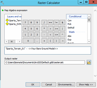
- Produce a canopy layer, use the Raster Calculator to filter the output from step 4 with the output from step 6.
Con( <<”output from 6”>> == 0, Int(<<”output from 4”>>), 0)
Make sure you critically evaluate the output of each step. “How do the parameters affect this model?” “Does this output differ from a previous run with differing model parameters? If so, how?”
One final suggestion. Take notes about what you are doing… What tool, input, output raster, parameter values, etc. You will not remember what you have done ten steps into the process.
Step By Step:
Step 1: Create a bare ground model: You might need to run this tool a couple of times with differing widths and heights. I ran the tool until there were no apparent tree rows in the terrain model. Smaller values will leave more detail (trees and other ground-level features) and larger values will produce a more general model of the ground.
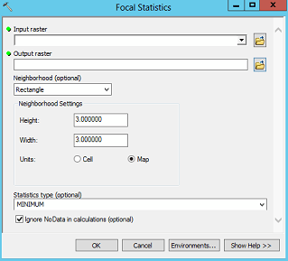
- Input Raster: Sparta_Terrain_01
- Output Raster: Sparta_BGM_<<width>>_<<height>>.img (save in your working directory)
- Neighborhood: Rectangle
- Height/Width: Use the same value for both width and height. You will need to adjust this to a size where the trees in the terrain model disappear. The tree canopies are around 0.5 to 1.5 meters in width. That is a good minimum starting point.
- Units: Map
- Statistics Type: Minimum
Step 2: Normalize the terrain: This process produces a flat plane. Unlike the original terrain model, pixel values are in terms of height above ground level.
- Call this NormalizedTerrain.img
- Make sure you save your output in your working directory
- Look at the min and max values. Do they make sense?
Step 3: Find tree canopies: Here, you are trying to find each tree’s apex. You are using a circle neighborhood because our targets are circular in shape. If your radius is too large, adjacent trees will be smudged together. If your radius is too small, you might introduce noise/phantom trees in the output.

- Input Raster: your normalized terrain
- Output Raster: CanopyModel.img
- Neighborhood: circle (you are looking for circle-shaped objects)
- Radius: select a radius small enough to isolate individual tree canopies
- Units: Map
Step 4: Segment your tree canopy. Segment Mean Shift is ArcGIS’ image segmentation routine. This process attempts to group similar pixels. Higher values for Spectral and Spatial Detail will produce more pleasing results.

- Input Raster: your canopy model
- Output Raster: my_trees.img
- Spectral/Spatial Detail: 20
- Minimum Segment Size: 5 (this is the smallest segment allowed; low number will allow many small noisy segments)
Change the Symbology to discrete colors when viewing this image (right-click on layer>Properties>Symbology>Discrete Color (left pane)).
Step 5: Mean filter non-tree area, part 1. Here, we are trying to remove the small segments while maintaining the large segments. This first step runs a rectangular window across the SMS image (Step 4) and calculates the mean. You want to use a window small enough to fit in your ‘tree’ segments but large enough to span those small non-tree segments. If you select an appropriate window size, the larger contiguous pixels will shrink slightly. The smaller non-tree segments, however, will turn into a sea of mixed pixels. Symbolize the output of this tool using a discrete color symbology.
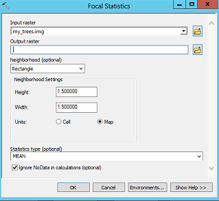
- Input Raster: my_trees.img
- Output Raster: FM_part1.img
- Neighborhood: Rectangle
- Height/Width: a value smaller than the one you used in Step 3;
- Units: Map
- Statistics: Mean
Step 6: Range filter non-tree area, part 2. Part 2 of the filtering process uses a focal statistics tool to calculate the RANGE. If all of the pixels in this window are the same value, then the range is 0. Select a window small enough to fit in your tree segments but large enough to span the small non-tree segments.

- Input Raster: FM_part1.img (layer from step 4)
- Output Raster: my_trees_range.img
- Neighborhood: Rectangle
- Height/Width: smaller value yields ‘more’ trees, larger value yields ‘smaller’ trees
- Units: Map
- Statistics: Range
Step 7: Produce tree canopy model. Display the output of this step using a classified symbology. Use two classes, 0 and all other values.

- Output Raster: Tree_segments.img
- The Raster Catalog command is:
Con(“<<output from Step 6>>” == 0, “my_trees.img”, 0) - This is an If/Then tool; if a cell in the output from step 6 = 0, give the new raster the value from the my_trees layer, else give the new cell a value of 0
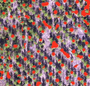
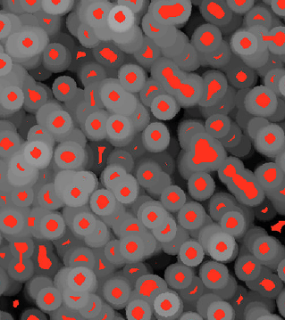
My First Run Output:
Unfortunately, the results of my first run appear to capture only some of the trees.
Compare the non-zero values in your Tree_segments.img layer with your normalized terrain (below).

Also, compare the non-zero values in your Tree_segments.img layer with your CanopyModel.img (below).
 SMS
SMS
Model refinement:
Think back to Step 3. You used a circular moving window (your choice of radius) to calculate the focal maximums across your normalized terrain model. The assumption here is the focal maximums represent a tree’s apex. It is evident from my example that my moving circular window was too wide. If I selected a larger moving window, I think I would have even fewer trees identified. To refine my output, I need to return to Step 3 and select a smaller window.
The refinement process is tedious so it might be a good idea to create a Step 3 – 7 model (using the Spatial Modeler). Open the Spatial Modeler (Geoprocessing > Spatial Modeler), drag the tools you used in Steps 3 – 7 and then connect each process. Double-click on each process in the model and fill out the dialog; ensure you change your output names.
Homework deliverable:
Run through this process once and evaluate your output. I’m certain you will find areas where the process successfully identified a tree and other areas where trees were missed. Zoom into an area where your process failed. Overlay the results of Step 7 on the aerial photo; symbolize the overlay so you can see the trees and then all other areas NoFill so you can see the aerial. Take a screen shot and paste it in a Word document.
Now, go back and refine your model. Take a screen shot of the same area and paste it into the Word document. Tell me what you did to refine your model. Was your refinement successful?