We’ll get back to project planning Friday. In the meantime, lets review Monday’s lab and spatial data modeling in general.
The most exciting phrase to hear in science, the one that heralds new discoveries, is not "Eureka!", but "That's funny..."
(Isaac Asimov)
In my case, the phrase is “…hmmm. That’s weird…”
Monday’s Spatial Model
The workflow went something like this:
Step 1: Focal Minimum to find the ground surface
Step 2: Normalize the terrain model
Step 3: Focal Maximum to find the tree apex (0.45m)
Step 4: Segment Mean Shift to group adjacent pixels with similar values
Step 5: Focal Mean to isolate the larg(er) homogenous groups of pixels from surrounding small(er) groups of pixels, part 1 (0.3m)
Step 6: Focal Range to further isolate the homogenous groups of pixels, part 2 (0.3m)
Step 7: Raster Calculator to mask the homogenous pixel groups you found in steps 5 and 6
And your spatial model might look something like this:
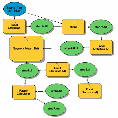
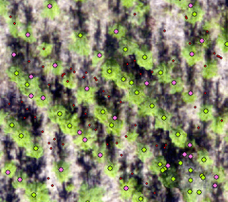
The result of my refined model from Monday identified groups of homogenous pixels in the original terrain model. Those homogenous pixels might represent a tree crown, or they might represent an area between the rows (screenshot below).
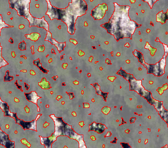
The larg(er) areas between the rows, the non-grey areas in the screenshot above, can be filtered out by:
- Select the 0-VALUE cells in the Step 7 output and convert them to a polygon (Raster to Polygon)
- Convert that polygon output to a point layer (Polygon to Point)
- Determine the normalized elevation for each point (Extract Values to Points).
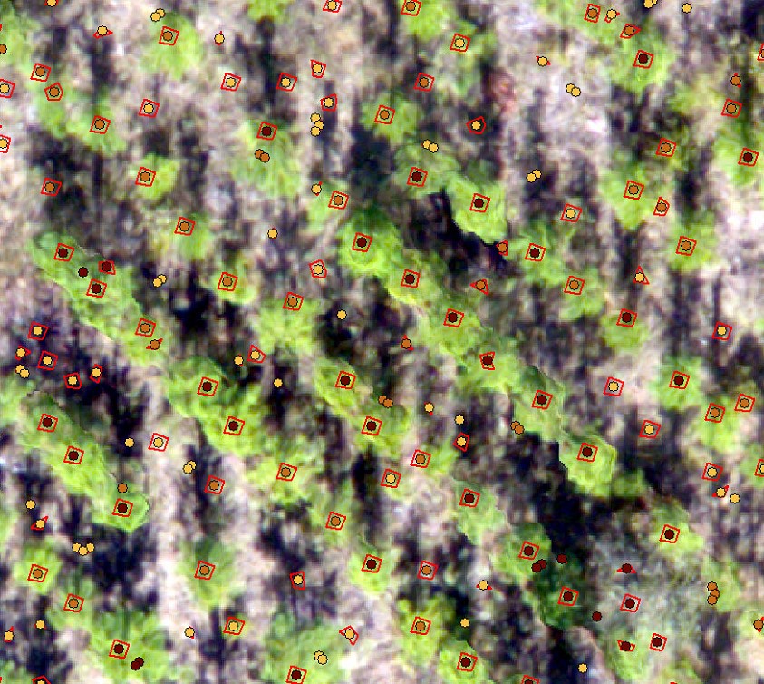
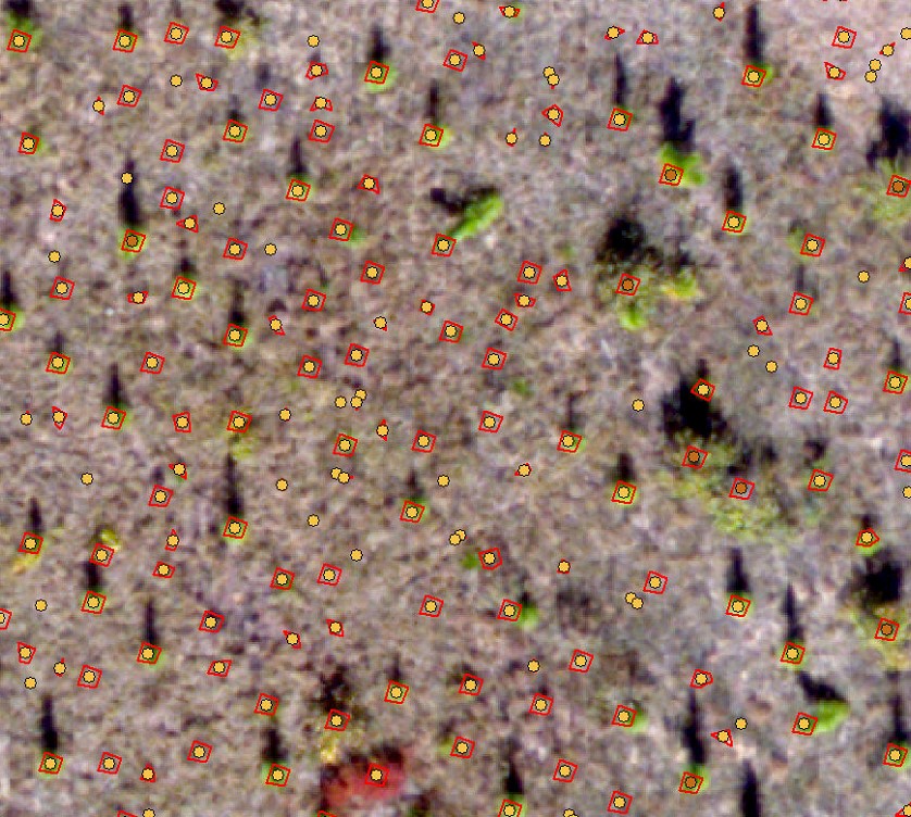
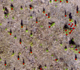
The results look like this:
However, I did find areas where this approach failed.
Model Simplification:
Recall that you used the Focal Statistics tool in Step 3 to find the tree canopy high-points. The process of assigning values to the new output raster flows something like below, where the maximum value from the 3×3 cell window is assigned to the pixel whose location is in the center of the 3×3 window

Cell values A1, A2, and A3 in the output raster do NOT reflect the crown apex. Their cell values in the new output will not be the largest values in the area. The remaining cells in this example, however, do capture that local maximum from Step 3. The cell values in our new output for the 3×3 cell area centered on the tree apex WILL be populated with the SAME, LOCALLY MACIMUM value.

In my model, I used a 0.45 meter moving window to calculate the Focal Maximum so I have a 0.45×0.45 meter area assigned the maximum (screen shot below) instead of a 3×3 cell area like above.

The Eureka Moment… SLOPE
After Step 3, I have a raster layer where I isolated and essentially expanded the local high spots (tree crowns) in the image. Out of curiosity, I ran the SLOPE command on this output which yielded this
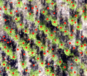
and this
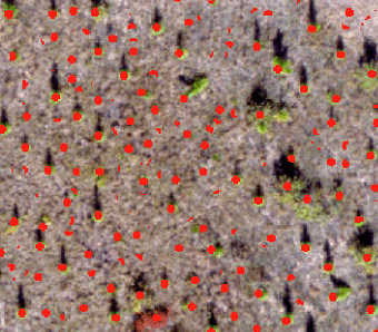
I finished the simplified, 3-step process, by using the
- RECLASSIFY command to change all 0 cells to 1 and every other value to NODATA, then ran the
- REGION GROUP command to group adjacent pixels into their own class, then
- Converted the output to a polygon layer using the RASTER TO POLYGON tool and then
- Converted the polygon to a point layer using the FEATURE TO POINT tool. I finished the process by
- Populating the point layer with the normalized elevation, Step 2 output, using the EXTRACT VALUES TO POINTS command
- ZONAL STATISTICS command to populate the Region Group output from above with the values in the Step 3 output raster, and then ran the
- RASTER TO POINT