In this lab, you will generate a point cloud and an orthophoto from photos captured during one of my UAV flights last November. You will use the LiDAR toolset in Global Mapper to generate a bare ground “terrain” model and a “surface” model (includes trees, stumps, buildings, etc).
———————————————————————————
Create a working directory on the C:\ Drive
Download lab data (HERE) and copy it over to your working directory
Unzip your data file. You should now have two folders; one named InputPhotos and another PhotoscanOutput
———————————————————————————
Open Global Mapper v19.1
- Set Coordinate System: Tools > Configure > Projection > UTM/Zone17/NAD83/METERS
- Save your project in the working directory you set up
Convert UAV photos to point cloud using the Pixels to Points tool
- File > Open Data Files load UAV photos
- File > Open Data Files load clpSG)Ortho.img
- Load Pixels-To-Points (PTP) tool (located on the LiDAR toolbar, last icon on the right)

- From the PTP tool
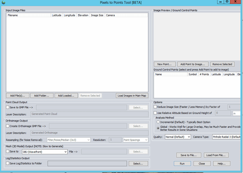
- Add Files: load the UAV imagery
- Point Cloud/Orthoimage/Mesh/Log Output: Save outputs in GMP (Global Mapper) format in your working directory
- Create Orthoimage GMP File
- Reduce Image Size: (use 8 to speed processing for lab) down-samples the original images which decreases processing time
- Analysis Method: means by which matching points are located on UAV photos
- Incremental: The Incremental method starts from two images, and progressively adds more, recalculating the parameters and locations of the points to minimize the error.
- Global: considers the keypoints across all images at the same time.
Output of Pixels To Points tool


Save your outputs in a common GIS-ready format:
- Right-click on the layer you want to export from Global Mapper > EXPORT… > select your file type > name your output & hit Apply/OK
- Save your point cloud as a LAS file
- Save your other raster layers as an ERDAS Imagine File
CONTINUATION of Monday’s lab…
Global Mapper is the second software that you have seen this semester that allows you to create an orthophoto and a point cloud from a series of photos (ReCap Pro is the other). While it appears that Global Mapper does have quite a bit of GIS functionality, we’ll be analyzing the output in ArcGIS and R.
Think back to Lab 7 and the Lab 7 Follow-up. The simplified locate-tree workflow we followed was:
- Focal Minimum to find the ground surface
- Difference original surface model and the focal minimum output
- Focal Maximum on output to find tree apex
- Generate slope
- Reclassify 0-slope as 1 (YES tree)
- Convert to polygon then polygon-to-point
Lets try this approach on Monday’s data… (In-class Demo)…
Now, in R…
https://cran.r-project.org/web/packages/lidR/lidR.pdf
#####load required R libraries
library(lidR)
library(raster)
#####Install Bioconductor
source("https://bioconductor.org/biocLite.R")
biocLite("EBImage")
library(EBImage)

#####specify my working directory
setwd("G:/UAV/SouthernGrowers/SmallSubset/out/")

#####read LAS file generated in Agisoft Photoscan, Global Mapper, etc...
my_data1<- readLAS("clpSoutheasternGrowers_PointCloud.las")
summary(my_data1)
my_data1bak<- my_data1  #####back up the original data file

#####classify ground layer
#####sequences used in the lasground command
ws = seq(0.75,3, 0.75) th = seq(0.1, 1.1, length.out = length(ws))
lasground(my_data1, "pmf", ws, th)
plot(my_data1, color = "Classification")

my_data1grnd<- my_data1  #####back up ground classification
####writeLAS(my_data1,"xxy.las")

#####compute DTM
dtm1 = grid_terrain(my_data1, res=0.9, method="knnidw", k=10, keep_lowest=TRUE)
dtm1r = as.raster(dtm1)
plot(dtm1)

#####normalize point cloud
##lnorm = lasnormalize(my_data1, method="kriging", k=10L)
lasnormalize(my_data1, dtm1)
#####my_data1 now contains the normalized heights
summary(my_data1)
plot(my_data1)
plot(dtm1)


#####create grid canopy
chm = grid_canopy(my_data1, res=0.25, subcircle = 0.2)
chm2 = grid_canopy(my_data1, 0.15, subcircle = 0.2)
chm2 = grid_canopy(my_data1, 0.05, subcircle = 0.025)
plot(chm2)
chm2 = as.raster(chm2)

#####smoothing post-process (2x mean)
kernel<- matrix(1,3,3)
chm2a = raster::focal(chm2, w=kernel, fun=mean)
chm2a = raster::focal(chm2, w=kernel, fun=mean)
raster::plot(chm2a, col=height.colors(50))

#####segmentation
crowns = lastrees(my_data1, "watershed", chm2a, th=0.25, extra=TRUE)
contour = rasterToPolygons(crowns, dissolve=TRUE)
tree = lasfilter(my_data1, !is.na(treeID))
##plot(tree, color="treeID", colorPalette=pastel.colors(200))

plot(chm2, col=height.colors(50))
plot(contour, add=T)

plot(tree)
#####Output new raster file called "ttyz.img"
raster::writeRaster(my_trees, filename="ttyz.img", format="HFA", overwrite=TRUE)