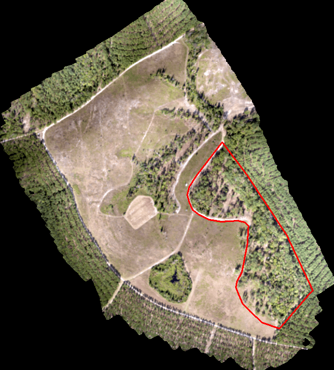
Today’s scenario. We need to perform a similar analysis on a site I flew last summer. We are only interested in the area outlined in red (screenshot below).
INPUT DATA:
- Input LAS: sp2_pcloud.las (DropBox Link)
- Processing extent: AnalysisUnit.shp
R WORKFLOW:
- Clip input data to processing extent
- Classify ground points
- Create bare ground model
- Normalize terrain model
- Create CHM
- Segment image
- Export
LAST WEEK’S CONTENT
#####Code from Lab 9
#####Install/Load libraries
source("https://bioconductor.org/biocLite.R")
biocLite("EBImage")
library(EBImage)
library(lidR)
library(raster)
#####Specify Working Directory
#####This should point to the directory in which your *.las resides
setwd("C:/temp/Nov30_2017/PhotoscanOutput/")
#####Read LAS file
#####https://rdrr.io/cran/lidR/man/readLAS.html
my_data1<- readLAS("clpSG_PointCloud_th001.las")
##make note of min/max X Y Z:
##make note of Num. of point records
summary(my_data1)
NEW CONTENT
#####!!!!!!!!!!!!!!!!!!!!!!!!!!NEW CONTENT!!!!!!!!!!
#####Read shapefile
pextent<- readOGR( ".","AnalysisUnit")
pe<- extent(pextent)
xmin<- pe[1]
xmax<- pe[2]
ymin<- pe[3]
ymax<- pe[4]

xlist<- c(xmin, xmax, xmax, xmin)
ylist<- c(ymax, ymax, ymin, ymin)
xylist<- cbind(xlist,ylist)

polyextent<- Polygon(xylist)
clp_mydat<- lasclip(mydat, polyextent)

plot(clp_mydat)
FROM LAB 9 (CLASSIFY GROUND POINTS)
#####Classify ground points
#####https://rdrr.io/cran/lidR/man/lasground.html
#####ws: sequence of window sizes to be used in filtering ground points
ws = seq(0.75,3, 0.75)
#####th: sequence of threshold heights above the surface to be considered a ground return
#####this step may take some time to run...
th = seq(0.1, 1.1, length.out = length(ws))
lasground(my_data1, "pmf", ws, th)
plot(my_data1, color = "Classification")
#####make a back up of the my_data1 object
my_data1_bak<- my_data1
FROM LAB 9 (COMPUTE DTM)
#####compute digital terrain model (DTM), this is the surface minus features sitting on top
#####https://rdrr.io/cran/lidR/man/grid_terrain.html
dtm1 = grid_terrain(my_data1, res=0.9, method="knnidw", k=10, keep_lowest=TRUE)
plot(dtm1)
#####process w/ smaller ground resolution
my_data1<- my_data1_bak
dtm2 = grid_terrain(my_data1, res=0.5, method="knnidw", k=10, keep_lowest=TRUE)
plot(dtm2)
FROM LAB 9 (NORMALIZE SURFACE)
#####normalize point cloud: subtract DTM from point cloud; value 0 represents ground-level
#####https://rdrr.io/cran/lidR/man/lasnormalize.html
lasnormalize(my_data1, dtm2)
#####my_data1 now contains the normalized heights
##make note of min/max X Y Z:
summary(my_data1)
plot(my_data1)
my_data1_bak2<- my_data1
FROM LAB 9 (CREATE CHM)
#####create grid canopy
#####for each grid, returns the highest point
#####https://rdrr.io/cran/lidR/man/grid_canopy.html
chm = grid_canopy(my_data1, res=0.25, subcircle = 0.2)
plot(chm)
my_data1<- my_data1_bak2
chm2 = grid_canopy(my_data1, 0.05, subcircle = 0.025)
plot(chm2)
#####notice the redefined canopies
chm2 = as.raster(chm2)
#####smoothing post-process (2x mean)
kernel<- matrix(1,3,3)
chm2a = raster::focal(chm2, w=kernel, fun=mean)
chm2a = raster::focal(chm2, w=kernel, fun=mean)
raster::plot(chm2a, col=height.colors(50))
FROM LAB 9 (SEGMENTATION PROCESS)
#####segmentation process
#####https://rdrr.io/cran/lidR/man/lastrees.html
crowns = lastrees(my_data1, "watershed", chm2a, th=0.25, extra=TRUE)
contour = rasterToPolygons(crowns, dissolve=TRUE)
tree = lasfilter(my_data1, !is.na(treeID))
plot(chm2, col=height.colors(50))
plot(contour, add=T)
#####write out to GIS image
raster::writeRaster(crowns, filename="crowns1.tif", format="HFA", overwrite=TRUE)