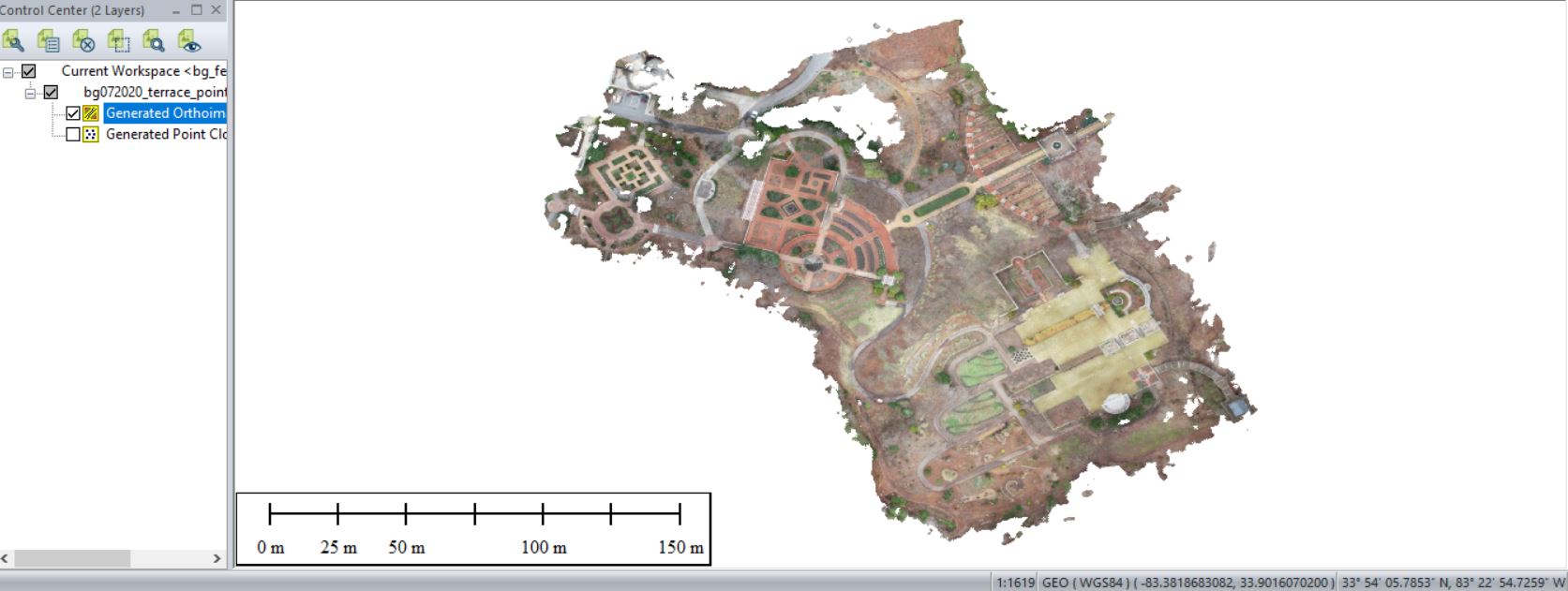
In this lab, you will be processing drone data acquired on February 07, 2020 at the terraced section of the UGA Botanical Garden. The photos were captured with the DJI Phantom 4 Professional using the DJI Ground Station software running on an iPAD mini; the drone was set to fly at a height of 75 meters above ground level with a sidelap of 80% and an endlap of 80%. The mission resulted in 84 photos.
The You will use the LiDAR toolset in Global Mapper to generate an orthophoto, a bare ground “terrain” model and a “surface” model (includes trees, stumps, buildings, etc).
———————————————————————————
Pre-processing data management: Data management is a necessity. Sooner or later, you will need to develop a data management strategy – one that allows you to quickly browse your data directory and know what is there and where it was captured. I try to create a project folder with separate subfolders to store the unprocessed drone photos, outputs, and any other existing GIS data.
- Create a working directory on the E:\ Drive called BotGarden_Feb072020. Also create a folder called InputPhotos and another folder called OutputData
- Download lab data (HERE) and copy it over to your working directory. The compressed file size is 706,494MB.
- Unzip your data file. Move photos ‘DJI_0029.JPG’ – ‘DJI_0104.JPG’ to the InputPhotos folder. You can delete the other photos.
———————————————————————————
Open Global Mapper v21.0
Pixels To Points Blue Marble Geo Help
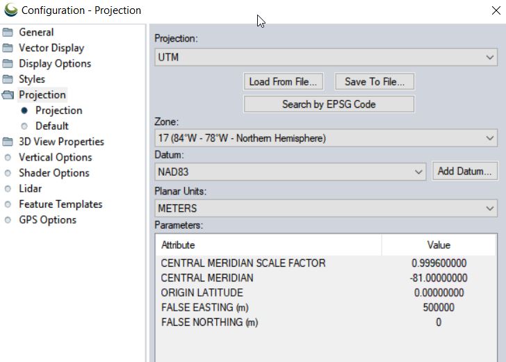
- Set Coordinate System: Tools > Configure > Projection > UTM/Zone17N/NAD83/METERS
- Save your project to your working directory
- File > Save Workspace As…
Convert UAV photos to point cloud using the Pixels to Points tool
- File > Open Data Files load UAV photos
- For context, load a basemap
- File > Download Online Imagery…
- Select World Imagery
- Save your workspace
- Load Pixels-To-Points (PTP) tool (located on the LiDAR toolbar, last icon on the right)

- From the PTP tool
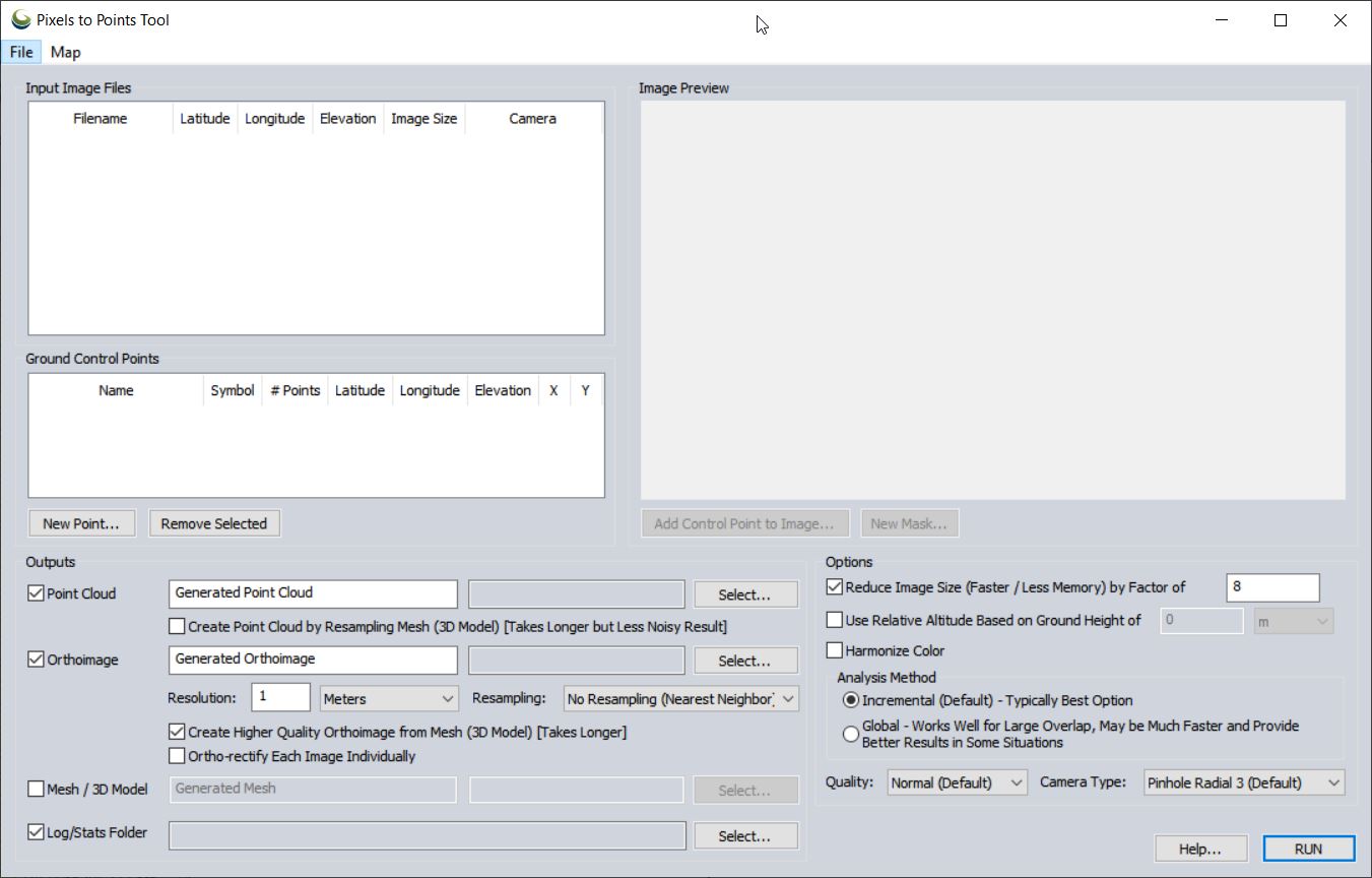
- Input Image Files: right-click > Add Loaded Pictures…
- Point Cloud/Orthoimage/Mesh/Log Output: Save “BG072020_pointcloud” (in GMP Global Mapper format) in your <working directory>\OutputData folder
- Orthoimage: Save “BG072020_ortho” in your OutputData folder
- Reduce Image Size: (use 8 to speed processing for lab) down-samples the original images which decreases processing time
- Analysis Method: means by which matching points are located on UAV photos
- Incremental: The Incremental method starts from two images, and progressively adds more, recalculating the parameters and locations of the points to minimize the error.
- Global: considers the keypoints across all images at the same time.
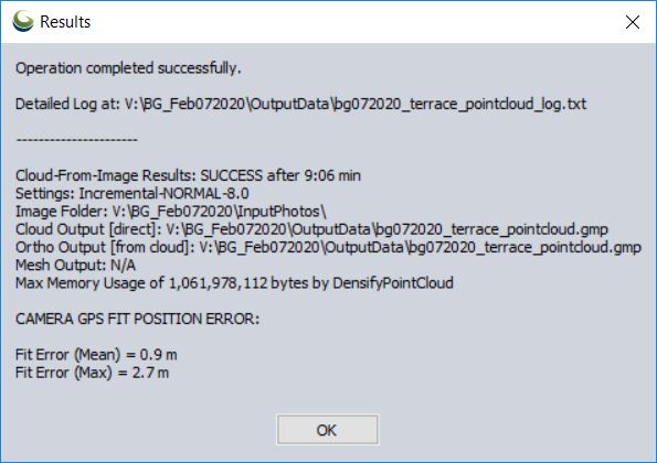
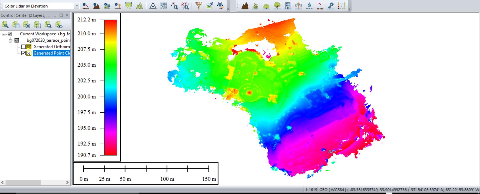
Output of Pixels To Points tool
Remove the individual drone photos (shift-select > right-click > remove…)
Save your outputs in a common GIS-ready format:
- Right-click on the layer you want to export from Global Mapper > EXPORT… > select your file type > name your output & hit Apply/OK
- Save your point cloud as a LAS file
- Save your other raster layers as an ERDAS Imagine File
Create surface and terrain models
Explore the Analysis > ‘Create Elevation Grid from 3D Vector/Lidar Data’ tool…
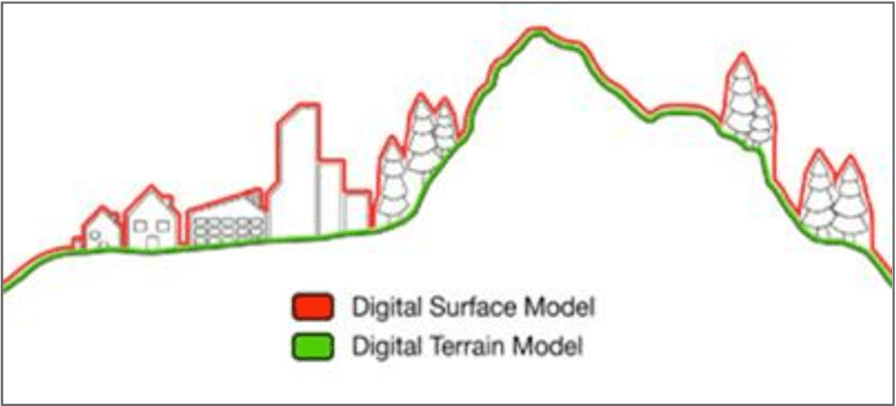
- Grid Method ‘Maximum Value – DSM’ to create a surface model
- Grid Method ‘Minimum Value – DTM’ to create a terrain model
Explore the Analysis > ‘Combine/Compare Terrain Layers’ tool…
We will work on this in a couple weeks…
CONTINUATION of Monday’s lab…
Global Mapper is the second software that you have seen this semester that allows you to create an orthophoto and a point cloud from a series of photos (ReCap Pro is the other). While it appears that Global Mapper does have quite a bit of GIS functionality, we’ll be analyzing the output in ArcGIS and R.
Think back to Lab 7 and the Lab 7 Follow-up. The simplified locate-tree workflow we followed was:
Focal Minimum to find the ground surfaceDifference original surface model and the focal minimum outputFocal Maximum on output to find tree apexGenerate slopeReclassify 0-slope as 1 (YES tree)Convert to polygon then polygon-to-point
Lets try this approach on Monday’s data… (In-class Demo)…
Now, in R…
https://cran.r-project.org/web/packages/lidR/lidR.pdf
#####load required R libraries
library(lidR)
library(raster)
#####Install Bioconductor
source("https://bioconductor.org/biocLite.R")
biocLite("EBImage")
library(EBImage)

#####specify my working directory
setwd("G:/UAV/SouthernGrowers/SmallSubset/out/")

#####read LAS file generated in Agisoft Photoscan, Global Mapper, etc...
my_data1<- readLAS("clpSoutheasternGrowers_PointCloud.las")
summary(my_data1)
my_data1bak<- my_data1  #####back up the original data file

#####classify ground layer
#####sequences used in the lasground command
ws = seq(0.75,3, 0.75) th = seq(0.1, 1.1, length.out = length(ws))
lasground(my_data1, "pmf", ws, th)
plot(my_data1, color = "Classification")

my_data1grnd<- my_data1  #####back up ground classification
####writeLAS(my_data1,"xxy.las")

#####compute DTM
dtm1 = grid_terrain(my_data1, res=0.9, method="knnidw", k=10, keep_lowest=TRUE)
dtm1r = as.raster(dtm1)
plot(dtm1)

#####normalize point cloud
##lnorm = lasnormalize(my_data1, method="kriging", k=10L)
lasnormalize(my_data1, dtm1)
#####my_data1 now contains the normalized heights
summary(my_data1)
plot(my_data1)
plot(dtm1)


#####create grid canopy
chm = grid_canopy(my_data1, res=0.25, subcircle = 0.2)
chm2 = grid_canopy(my_data1, 0.15, subcircle = 0.2)
chm2 = grid_canopy(my_data1, 0.05, subcircle = 0.025)
plot(chm2)
chm2 = as.raster(chm2)

#####smoothing post-process (2x mean)
kernel<- matrix(1,3,3)
chm2a = raster::focal(chm2, w=kernel, fun=mean)
chm2a = raster::focal(chm2, w=kernel, fun=mean)
raster::plot(chm2a, col=height.colors(50))

#####segmentation
crowns = lastrees(my_data1, "watershed", chm2a, th=0.25, extra=TRUE)
contour = rasterToPolygons(crowns, dissolve=TRUE)
tree = lasfilter(my_data1, !is.na(treeID))
##plot(tree, color="treeID", colorPalette=pastel.colors(200))

plot(chm2, col=height.colors(50))
plot(contour, add=T)

plot(tree)
#####Output new raster file called "ttyz.img"
raster::writeRaster(my_trees, filename="ttyz.img", format="HFA", overwrite=TRUE)